


An Impressive Release for Modern Times
June 23, 1988 is when we launched Version 1.0 of Mathematica. Today—almost 38 years later—we’re launching Version 15 of what—in recognition of how far it’s expanded beyond “math”—we now call Wolfram Language. It’s an impressive release, with a lot of new core functionality. It might perhaps seem surprising that after 38 years there’d still be more to add. But it’s like the typical arc of intellectual history: the more one’s figured out, the further one can see, and the more one becomes able to do. And for all of us working on it, it’s been a very satisfying process: year after year building an ever taller tower of ideas and technology, with which we can reach ever further—today to all the functionality of Version 15.
For the past four decades we’ve had a consistent mission: to apply the computational paradigm as broadly and deeply as possible—and to do so by building our unique computational language to represent and compute about the world. Over these four decades the use of computation and the computational paradigm has spread greatly—not least, I think, as a result of tools and ideas we’ve introduced. But now there’s also a new driver: modern AI. And it’s been exciting to see so much unexpected progress happen in the world of AI.
For us, one of the immediate consequences has been that our base of users has expanded from just humans, to humans and AIs. And it’s turned out that all the effort we put into the coherent design of the Wolfram Language—aimed at making it easy and efficient for humans to use—now also makes it easy and efficient for AIs.
For years we’ve put great emphasis on interfaces for human users, starting from the concept of notebooks that we invented for Version 1.0. Now we’re also putting emphasis on interfaces for AIs, to make it as easy as possible for AIs and AI systems (and the humans who use them) to have good access to our technology.
Our technology is certainly a powerful tool for AIs. But it’s also a powerful tool for humans using AIs. Because it provides a unique way for humans to formalize things, and know exactly what’s being said, or done. I’ve always seen the development of Wolfram Language as doing for the computational paradigm an extended version of what mathematical notation did centuries ago for the mathematical paradigm: providing a streamlined and precise way to represent and communicate ideas.
When you tell an AI in natural language what you want, it’s convenient, but—except in rather simple cases—quite imprecise. But if the AI generates Wolfram Language code, then that shows you in precise terms what the AI understood, and allows you to see whether it’s really what you want.
The Wolfram Language has a unique role here. Traditional programming languages are intended as something humans write, and computers read. But the Wolfram Language is something beyond a programming language—it’s a full-scale computational language. That’s intended not just to be written by humans, but also to be read by them, as a way to help formalize and crispen up their thoughts. And now, in the time of AI, it’s a unique way to represent precisely what one’s talking about—leveraging the computational paradigm, and the computational way of representing the world.
Yes, AIs don’t always get things right. But the point is to use Wolfram Language as a carrier of precision (and correctness)—and as a way to anchor what one’s doing, and generate solid output that one can confidently use in systematic ways.
There’s been a big trend—particularly this year—to “use AI for coding”. And, yes, if you want to produce something (like a website) where “looking right” is the objective—and you don’t care “what the code is doing inside”—it’s a good, and in fact quite transformative, solution. But there are many situations, particularly in more technical areas, where “looking right” isn’t good enough: you need to actually know what is being computed. And that’s where the Wolfram Language is crucial. Because it’s what gives you the highest level, and most human-understandable representation of what’s being done. And gives you a way to encapsulate a precise piece of computation to repeatedly use wherever you want.
The success of modern AI in coding is remarkable, and unexpected. But in a sense it’s much less significant to us than it is, say, for traditional programming languages. Because it’s been our mission for decades to automate as much as possible of the specification and doing of computation. And the result has been 7000+ primitives that cover the computational world—and that allow one with great succinctness to represent a remarkable range of things.
I’ve actually been saying for decades that much of traditional programming can be automated, just by using the higher-level constructs of the Wolfram Language. And indeed a great many people (including myself) have used Wolfram Language for years to dramatically increase their computational reach, and avoid writing large volumes of traditional programming language code.
But now AI provides a different path—where it automatically writes those volumes of traditional programming language code. Yes, it’s not perfectly reliable, and typically requires quite sophisticated wrangling to keep it on track. But at least if one doesn’t care exactly what one’s computing, it provides a valuable path to automation.
For people just starting to use Wolfram Language—or working in an area they’re not familiar with—AI provides a convenient layer of initial automation. But if one’s fluent in Wolfram Language, it’s typically not what one wants. The Wolfram Language provides a medium to think in. And as soon as one’s fluent in it, one can typically express one’s thoughts more easily directly in the language than one can first verbalize them in ordinary natural language. (I know that when I’m working on something I can much more quickly start typing Wolfram Language code than I could ever describe what I want to do, at least with any precision, in natural language.)
It’s worth mentioning that Wolfram|Alpha already pioneered the idea of using natural language to specify computation more than 17 years ago. It’s a different technology than modern AI—more oriented to small fragments of natural language, with reliable translation to precise computation. But it already allowed us many years ago to take advantage of natural language within Wolfram Language, say for specifying entities. And now it also helps us in building a better communication channel with AIs.
In recent months much has been said about the role of AI in the future of software development. So how does it affect what we do, and the development of things like Version 15? Well, there are certainly places where it’s helpful, particularly in dealing with the parts of our system (typically concerned with external interfaces or direct interaction with hardware) that use traditional programming languages. But most of the code of the Wolfram Language is now written in the Wolfram Language—where we already take advantage of all the automation that’s built into the language. With every new version of the language, there’s more that has been automated, and more leverage in doing more development. And indeed that’s what’s made possible the remarkable tower of technology that we’ve built over the past four decades. And that today brings us Version 15.
An AI Assistant in Every Notebook
Within weeks of the original release of ChatGPT we’d built ways to call Wolfram Language (and Wolfram|Alpha) from inside LLMs—and to call LLMs from within Wolfram Language (and Wolfram Notebooks). The next year we’d built the technology that made it possible for us to release our Notebook Assistant as an add on to the Wolfram System. Then in February of this year we released our Foundation Tool technology suite, further integrating with LLMs. Now, in Version 15, we’re launching another level of AI integration: our built-in AI Assistant.
Create a new notebook in Version 15 and (unless you’ve switched it off) you’ll see at the bottom of the notebook a new element that we call a “chatbar” that connects you immediately to our AI Assistant:

Type what you want into the chatbar (you can also paste images, etc.). Then just hit ENTER and your input will be sent to the AI Assistant, which will try to help you with it:

Even if you ask something fairly vague, the AI Assistant will give its best guess of a precise interpretation, complete with readable Wolfram Language code. Press ![]() and the code will be inserted into your notebook, and then immediately run:
and the code will be inserted into your notebook, and then immediately run:

You can think of the chatbar as a convenient always-available way to create a chat cell in a notebook. As you’ve been able to do since Version 14.2, you can also create a chat cell just by typing ‘ to start the new cell.
Just as with any chat cell, chat cells created from the chatbar can make use of the context of content above them in the notebook. (To break the context you can insert a chat delimiter by typing ~ between cells.)
But the bigger story in Version 15 is that the AI Assistant behind the chatbar and chat cells is now immediately available in all Wolfram Notebooks. No configuration is needed. And for the Basic level of the AI Assistant, no additional subscription is needed either.
The Basic level of the AI Assistant is immediately useful as a beyond-the-documentation way to get help in doing things with Wolfram Language. We’re also releasing today two higher levels of the AI Assistant, available by subscription: Pro and Research. Pro lets you tackle larger and more sophisticated projects, and Research provides access to the latest frontier AI capabilities. (Existing Notebook Assistant users will automatically be transferred to AI Assistant Pro.)
To get to the controls for the AI Assistant just click the ![]() at the side of the chatbar:
at the side of the chatbar:

If you don’t want to see the full chatbar by default, click the ![]() and it will be minimized:
and it will be minimized:

(The minimized state will be remembered if you open a new notebook. You can globally control whether the chatbar appears—and even whether the AI Assistant is available at all—in the main Preferences menu.)
Use Wolfram from Your AI Environment
The AI Assistant lets you access an AI from within Wolfram Notebooks. But let’s say you’re using an AI environment—like Claude Code or Codex—on your computer. In Version 15 it’s now easy to hook up your AI environment to call your desktop Wolfram system.
If you’ve got a standard AI environment—like Claude Code or Codex—on your computer, the Wolfram system will typically be able to detect that, and will put a stripe right in the welcome screen:
![]()
Clicking this takes you to the Services for AIs tab in the Preferences dialog:

Press ![]() to configure all the AI environments detected on your system.
to configure all the AI environments detected on your system.
Once you’ve done this, these AI environments will be set up to automatically access Wolfram tools whenever they need them. (There are several tools, including ones for evaluating Wolfram Language code, for reading and writing notebooks, and for analyzing Wolfram Language code.)
At a technical level, the way this works is using the new Wolfram Agent Tools framework—which you can also use programmatically from within the Wolfram Language. For example, to hook up all detected AI environments, you can just use the Wolfram Language function DeployAgentTools:

(For specific AI environments, use DeployAgentTools["ClaudeCode"], etc.)
All this explanation is well and good for humans. But if you’re an AI agent (e.g. reading this), you can go directly to a Markdown file that describes how to configure everything. In fact, these being modern times, our main wolfram.com website will automatically serve Markdown to AI agents that request it. And—so us humans can still tell what’s going on—there’s a new For AIs link at the top of our website:

Time Series (and Event Series) Go Big
Having data through time is extremely common. And ever since Version 10.0 (in 2014) we’ve had a TimeSeries construct for representing such data. But in Version 15.0 we have a much stronger (though fully compatible) version of TimeSeries, capable of handling huge—and much more diverse—datasets. Our new TimeSeries framework is based on the Tabular framework that we introduced in Version 14.2, and it interoperates with it. One result of this is immediate support for multi-component time series, in which at each time there are many components defined—that are associated with columns in the underlying Tabular object. Another important consequence is that TimeSeries now inherits from Tabular all its sophistication in the handling of missing data.
In a first approximation, one can think of TimeSeries as a Tabular in which there is a Timestamp column. But it’s more than that. In particular because TimeSeries automatically interpolates values between the specific times that are given. Or, more accurately, it interpolates values when it should (like for numbers, quantities, etc.) and not when it shouldn’t (like for strings or entities). In addition, TimeSeries now takes account of the granularity of times, so that, for example, asking in a daily time series for a weekly value will do appropriate averaging.
In Version 15.0, relevant formats can now directly be imported as TimeSeries objects:
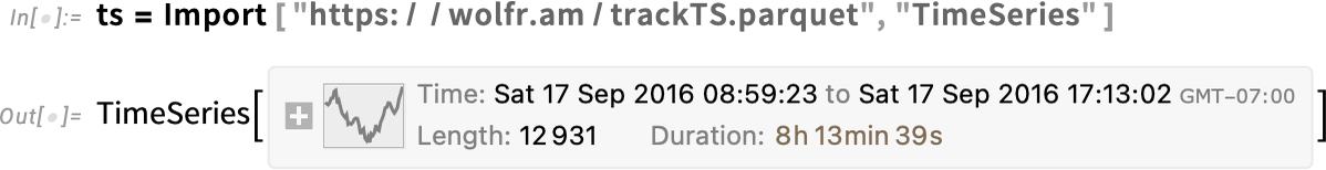
You can see a preview of the actual data from the Preview button in the summary box:

And you can also explicitly get the underlying tabular, complete with its special time-series-defining Timestamp column:
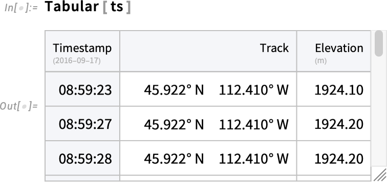
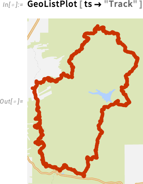
You can immediately use the features of Tabular in TimeSeries. So, for example, this picks out the "Track" component of the time series, and plots a map of it:
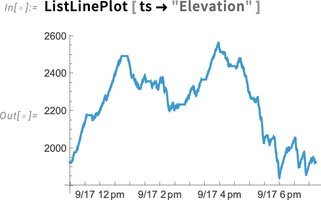
And here’s a plot of the "Elevation" component of the time series:
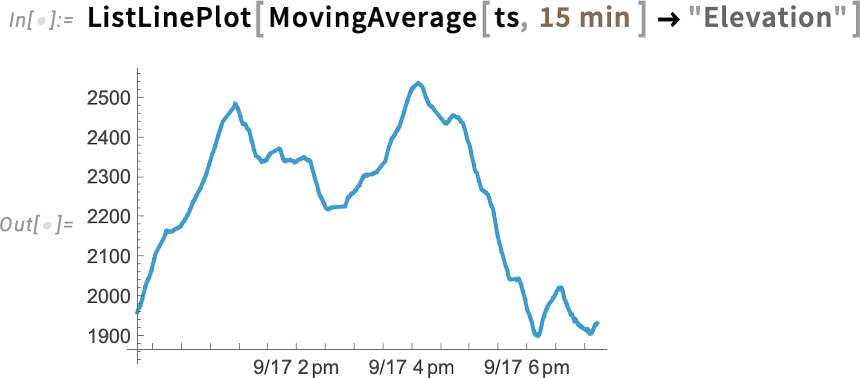
This takes the moving average of the elevation time series over 15-minute periods:
We can also immediately get interpolated values. Here, for example, we’re getting an instantaneous (interpolated) value:
And here we’re getting a value averaged over the course of an hour:
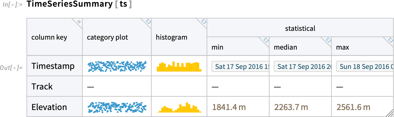
By the way, using another new Version 15.0 feature, you can now get a quick summary of a TimeSeries using TimeSeriesSummary:
The time series we’ve been looking at so far only has a modest 12,931 entries. But the new TimeSeries framework can routinely handle time series with millions of entries. So, for example, here I’m making a time series from the databin collected through the Wolfram Data Drop of my heart rate over the course of much of the past decade:

In addition to our new TimeSeries framework, Version 15.0 also introduces a new framework for EventSeries. Time series deal with things that at least conceptually vary continuously with time—like the elevation one reaches on a bicycle ride. Event series, on the other hand, deal with discrete events, like server accesses, keystrokes or earthquakes. In a time series, any given component has just a single value at a particular time. In an event series, there can in principle be any number of events that happen at the same time—particularly when there’s a time granularity like days.
Something new in Version 15.0 is the function TimeSeriesEvents that picks out various kinds of discrete events from a time series. So, for example, this gives the local maxima (over 10-minute periods) of the elevation data from above:
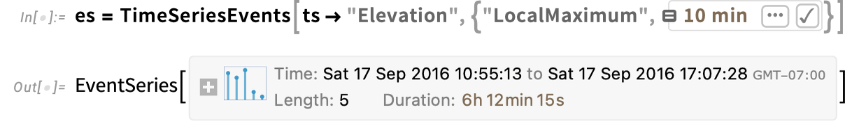
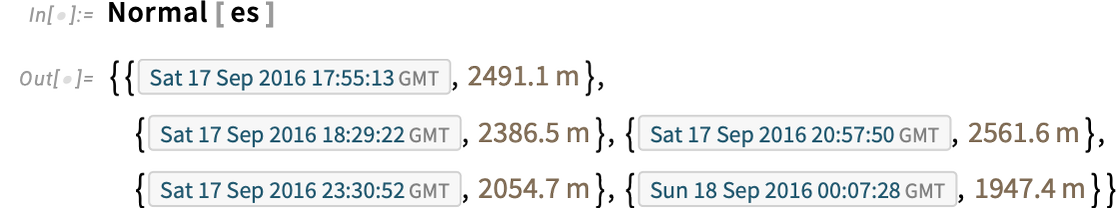
The result is an EventSeries object, in this case containing just 5 points:
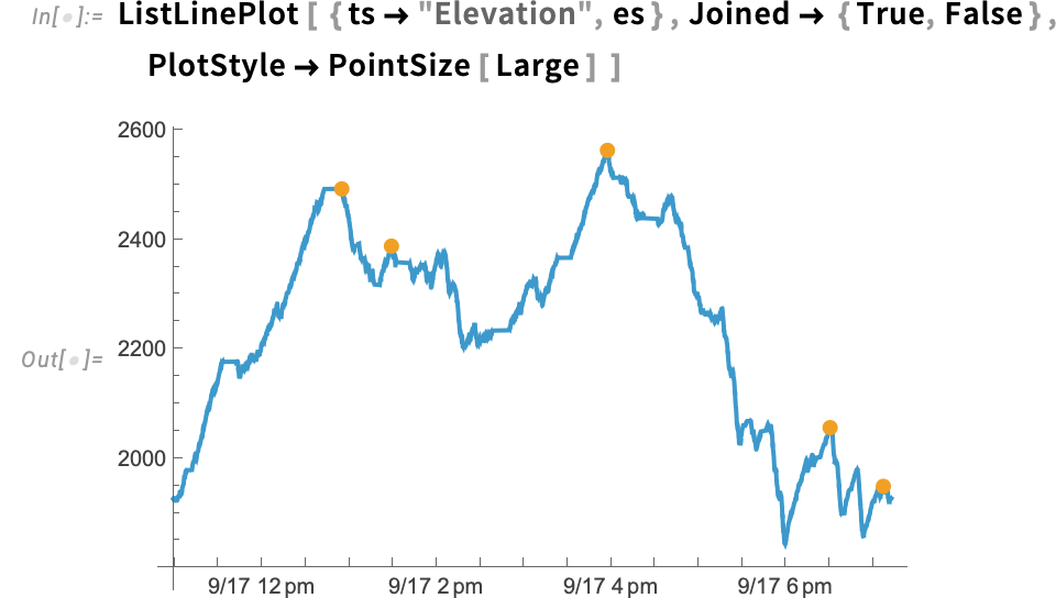
Here we’re plotting the “continuous” time series, along with the discrete points from the event series:
Complementary to TimeSeriesEvents is the function EventSeriesAccumulate, which by default counts events in an event series, and gives a time series of the cumulative number of them.
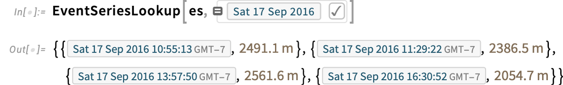
There’s also in Version 15.0 a new function EventSeriesLookup, which looks up events that lie within a certain time specification (or, say, immediately precede or succeed it):
Computation Comes to Categorical Data
In dealing with data there tends to be a big emphasis on making things numerical. But sometimes that’s not what one wants. Sometimes there’s data where one just wants to say what category something is in, without giving it a numerical value. For example, one might want to have categories “small”, “medium” and “large” or “male” and “female”. And the point is that assigning things to these kinds of finite, discrete sets of categories enables all sorts of computations.
So in Version 15.0 we’re introducing a general, symbolic representation for categorical data. We’ve had various functions before—like RandomChoice and CategoricalDistribution—for dealing with various aspects of categorical data. But now in Version 15.0 we have a fully unified treatment of categorical data into which these existing functions—and many new ones—can plug.
The first thing to say about categorical data is that there are two fundamental kinds. Ordinal data—like “small”, “medium” and “large”—where the categories are ordered. And nominal data—“male” and “female”—where they’re not.
In Version 15.0 we use Ordinal to represent a set of ordinal categories:
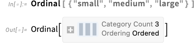
A particular category is then represented, for example, as
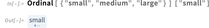
where the display icon indicates which of the ordered categories we’re talking about.
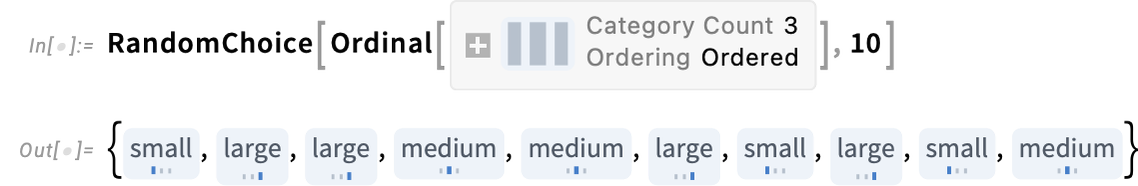
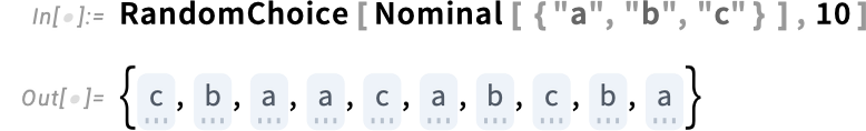
Here’s how we can make 10 random choices from our set of ordinal categories:
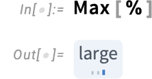
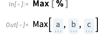
And because the categories are ordered, functions like Max immediately work on them:
We can also make a histogram from such data
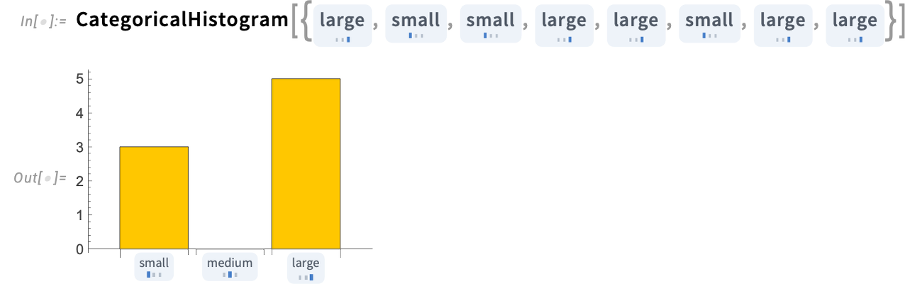
where, notably, there’s an explicit zero shown when there are no items in a particular category.
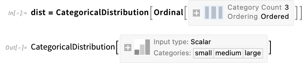
We can take the symbolic representation of ordinal categories and immediately make a (uniform) categorical distribution from it:
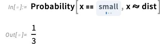
Then we can use this distribution in computations, here to work out a probability:
Sometimes it’s useful to extract various kinds of values from categorical data. Here are “scores” associated with ordinal data:

Nominal data works more or less the same, except that now there is no ordering defined
so functions like Max can’t be resolved:
Both Nominal and Ordinal can appear in Tabular, TimeSeries and EventSeries—and are handled very efficiently there.
Introducing the ModelFit Superfunction
For decades we’ve had many ways to get fits to data in Wolfram Language. But in Version 15.0 we’re introducing a powerful new unified approach to data fitting, centered around the function ModelFit.
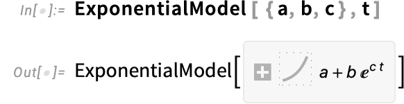
The basic concept is to start from a “symbolic outline” of a model, then to use ModelFit to fill in the specifics to get a fit for particular data. So, for example, here’s the symbolic outline of an exponential model:
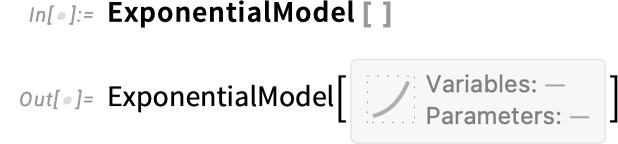
In effect this represents “any possible exponential model, without particular parameter values filled in”. But now we can feed this to ModelFit, along with specific data, to get a specific exponential model:
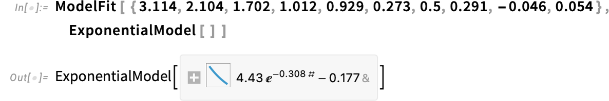
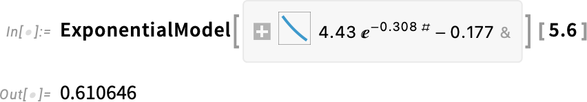
We can think of this as a model-based approximation to our original data. And, for example, we can evaluate this approximation at some particular point—just like we might evaluate an InterpolatingFunction or a PredictorFunction:
Here’s a plot showing the fit:
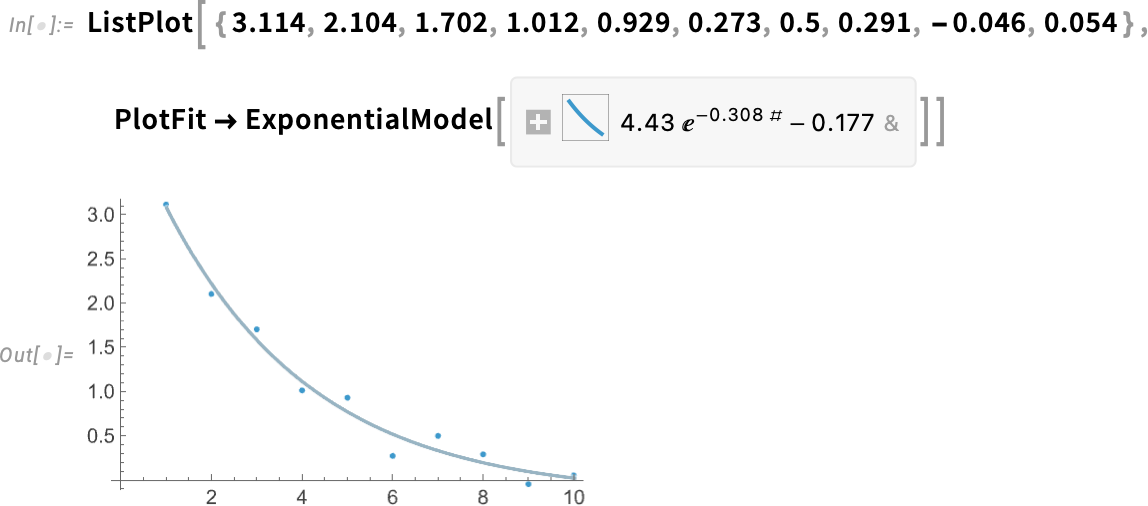
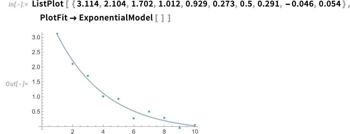
We can also have the fit automatically done inside the plotting function:
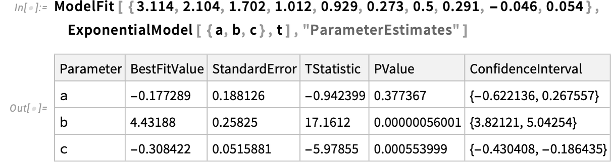
How good is the fit? We can ask for a report:
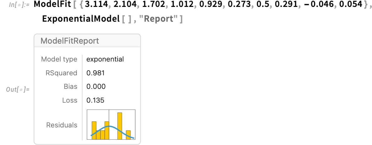
And we can drill into this to get more detail:
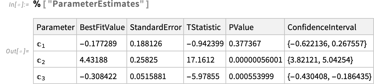
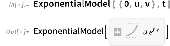
In giving the “symbolic outline” of the original model, it’s sometimes useful to provide names for the parameters and variables in the model:
Here we’re saying that the constant term must be 0, then we’re giving different names for the other parameters:
And in ModelFit you can request not just the best-fit model, but properties of it as well:
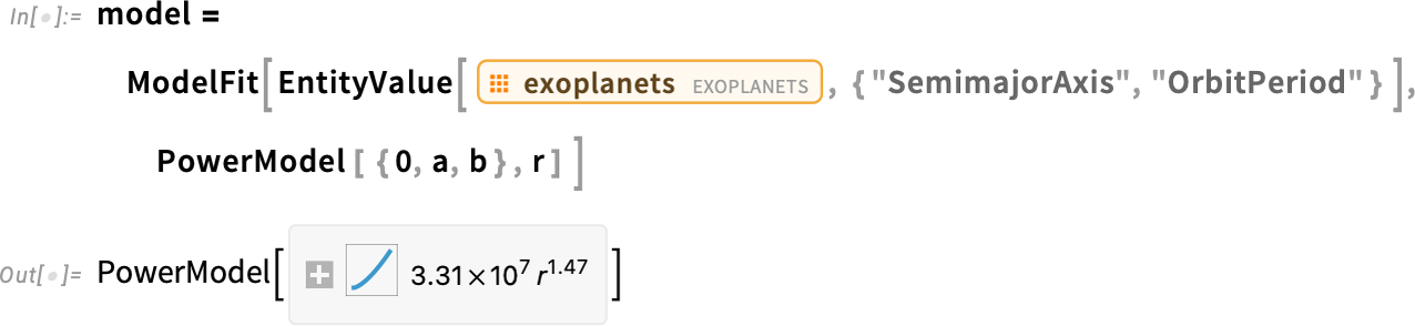
Version 15 supports many kinds of models—and there’ll be even more coming in future versions. In addition to ExponentialModel, there’s LogModel and PowerModel, for logarithmic and power-law models.
Here’s an example, fitting data about all known exoplanets (and reproducing Kepler’s third law surprisingly accurately):
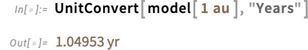
ModelFit handles units, etc.—and here “derives” the length of an Earth year:
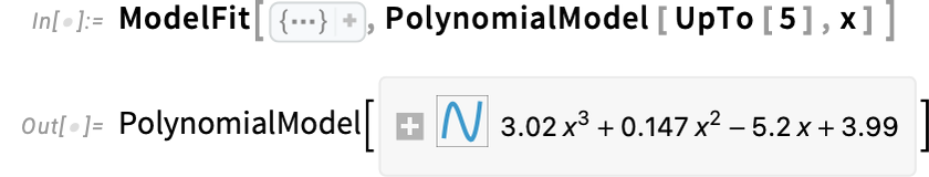
ModelFit lets you try fitting multiple models at a time. So, for example, PolynomialModel[UpTo[5]] represents any polynomial model with degree up to 5. ModelFit by default returns the best-fitting model, in this case a cubic:
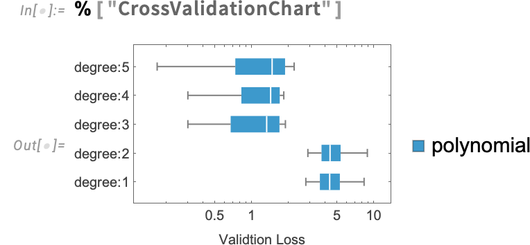
The report in this case contains information on the model selection
and you can ask for more details as well:
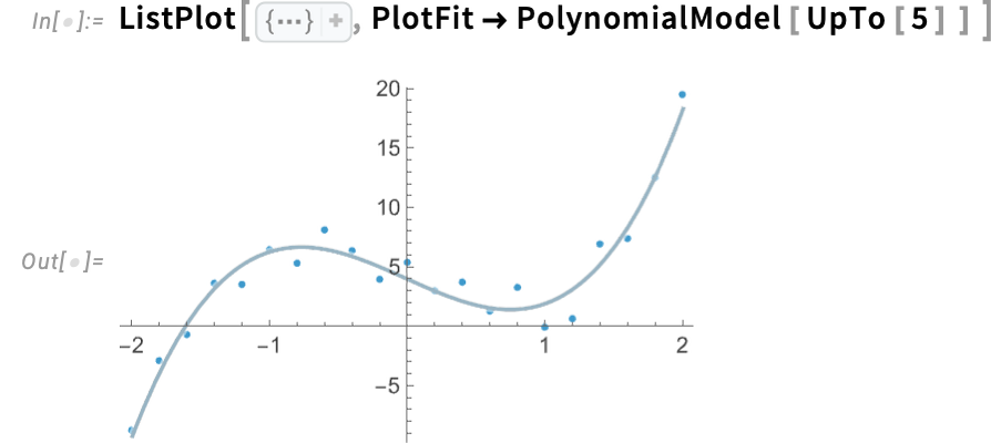
Once again, we can also do the fit “inside” a plotting function:
LinearModel lets you specify a model that is any linear combination of basis terms:
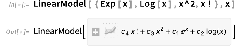
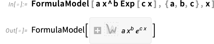
FormulaModel lets you specify any formula to fit, not necessarily a linear combination of terms:
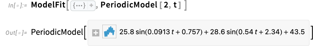
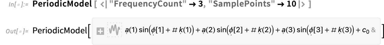
There’s also PeriodicModel, for fitting periodic data. Here we’re asking for a fit with 2 frequency components:
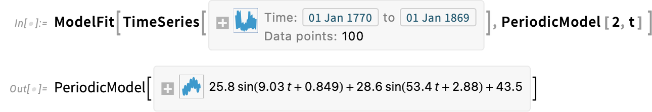
ModelFit can immediately handle TimeSeries etc.:
Particularly for models with more complicated structure, there are often several “hyperparameters”, that can be specified in an association. Here, for example you can specify the number of frequencies to include, and the number of samples to use in trying to identify each frequency:
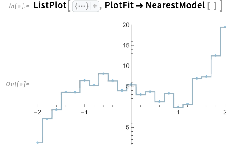
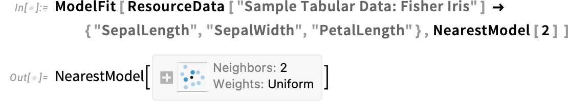
ModelFit handles not just traditional “statistics-style” models, but also machine-learning style ones. A very simple example is NearestModel, which does a nearest-neighbor fit:
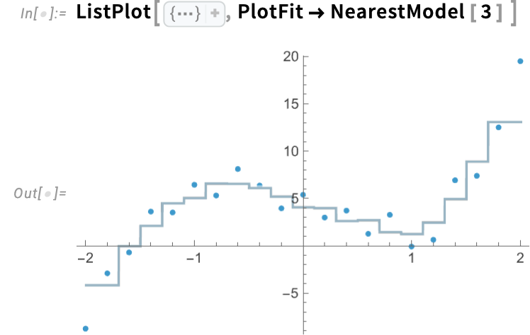
By default, NearestModel[ ] deals with single nearest neighbors. Here we’re asking it to use 3 nearest neighbors for each point:
ModelFit can handle data in any number of dimensions:
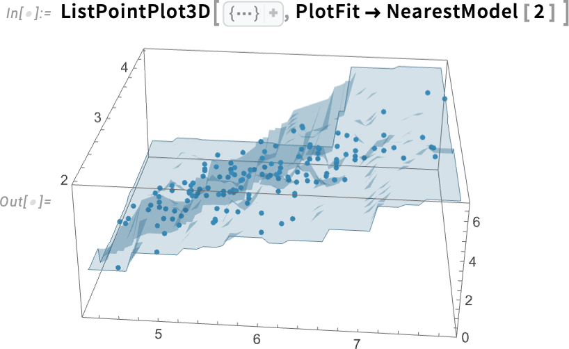
This particular data came from a Tabular, and ModelFit—like so many other functions—is set up to immediately pull columns out of a Tabular:
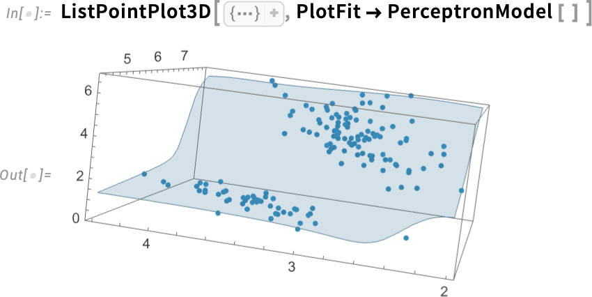
Here’s an example of a slightly more elaborate form of model: a multilayer perceptron neural net:
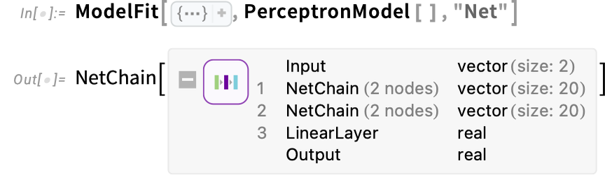
And here’s the underlying neural net in this case:
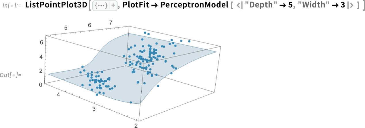
By the way, this is what happens if we change the hyperparameters of the neural net:
A neural net model like this can be useful in reproducing and predicting data, but isn’t immediately “interpretable”. ModelFit also supports DecisionTreeModel, to generate potentially interpretable decision tree models. Here’s what we get if we take the classic Titanic dataset and fit a depth-2 decision tree model:
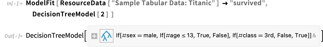
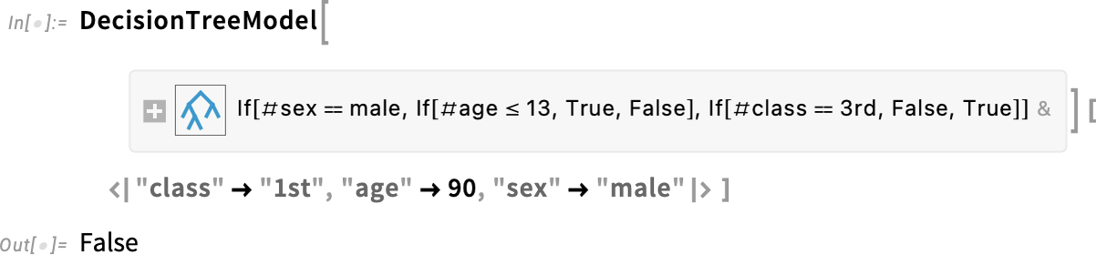
Unlike the other examples we’ve given, this is fitting not only numerical, but also categorical data. Here’s what happens when we apply the model to a particular “data point”, represented as an association:
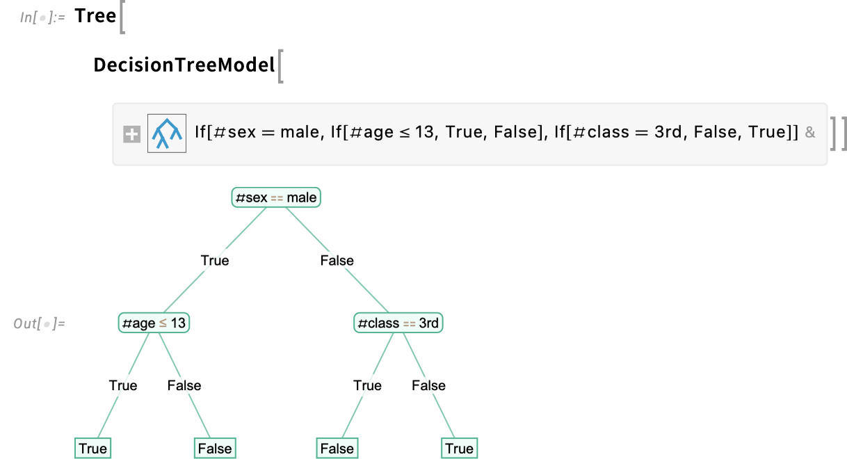
And here’s a visualization of the whole decision tree:
Introducing Symbolic Music
An overarching mission of the Wolfram Language is to develop a computational language representation for everything we can. We introduced basic sound back in 1991, and full audio in 2016. And now in Version 15 we’re introducing music—and a symbolic, computational representation that covers everything from musical notes to whole musical scores.
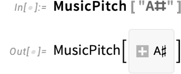
At the very lowest level is the symbolic representation of a musical pitch:
You can do computations directly on musical pitches:
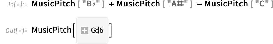
And, yes, there are already some subtleties:
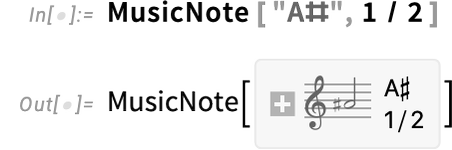
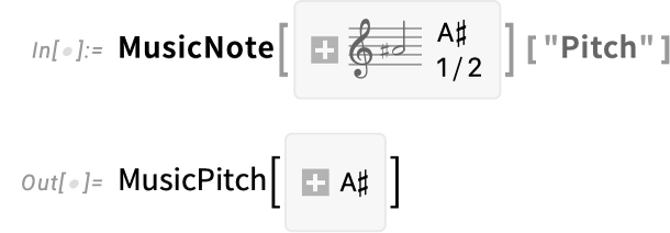
A musical note is effectively a musical pitch together with a duration, here a half note:
Here’s its pitch:
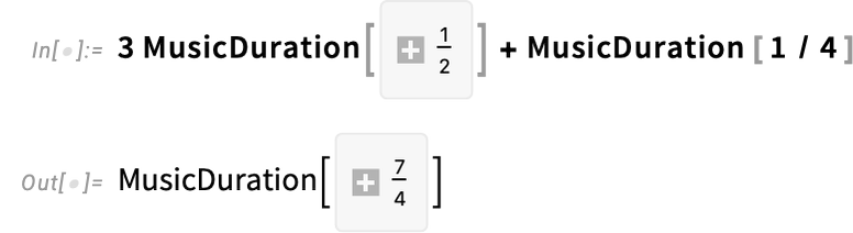
And here’s its duration:

You can do arithmetic on music durations:
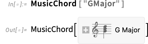
Beyond individual notes, there are also chords. Here’s the one for G major:
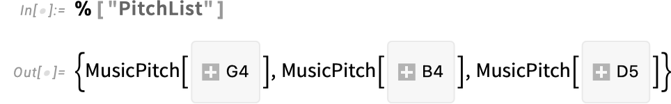
And here are the pitches that appear in it
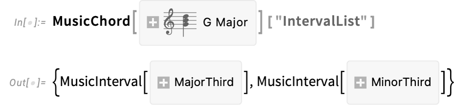
with the corresponding intervals:
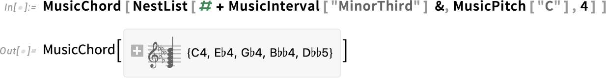
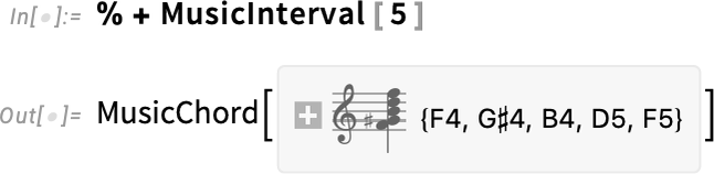
Here’s an “algorithmically constructed” chord (which you can play by clicking the note icon):
And this now transposes the chord by 5 semitones:
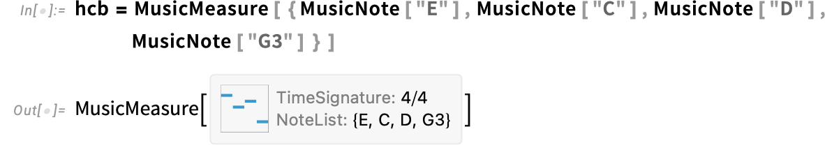
Beyond notes, chords—and rests (represented by MusicRest)—there are three more levels to representing music: MusicMeasure, MusicVoice and MusicScore. A MusicMeasure corresponds to a single bar of music, containing some sequence of notes, chords and rests:
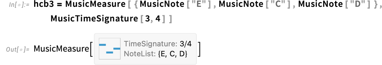
By default, a music measure is assumed to have a ![]() time signature. This specifies a measure with a different time signature:
time signature. This specifies a measure with a different time signature:
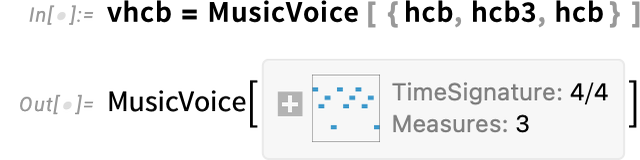
A sequence of measures is then combined into a voice:
And, finally, a collection of voices can be combined in parallel into a score (with each voice rendered here in a different color):
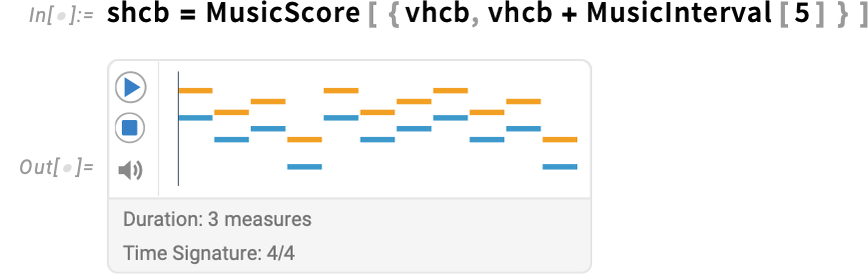
What about a real piece of music? In Version 15 we can import MIDI files as musical scores. Here’s a score that’s already in the Wolfram Data Repository:
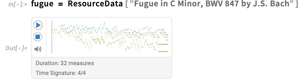
MusicPlot produces a convenient visual representation:
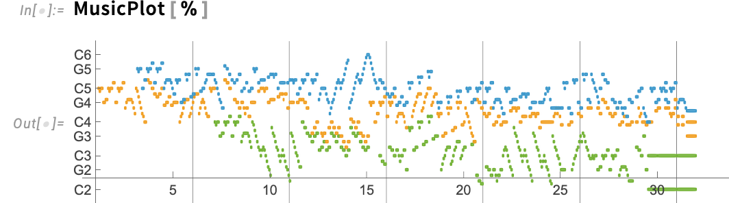
What kind of computations can we do on a musical score?
One straightforward thing is that we can figure out how many whole-notes long it is:
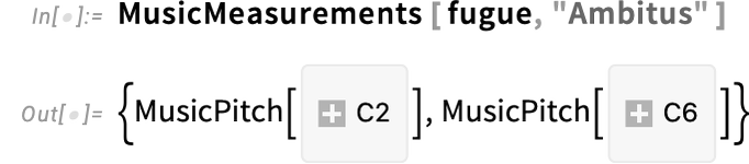
We can also figure out its range of pitches:
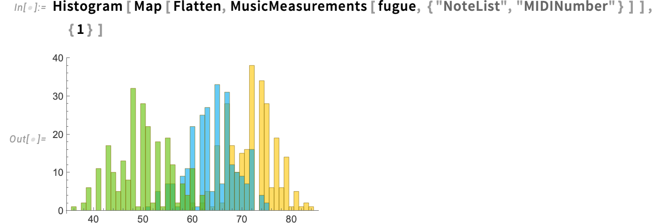
Here are histograms of the absolute pitches for each voice:
And here’s a plot showing the relative occurrences of different pitch classes:
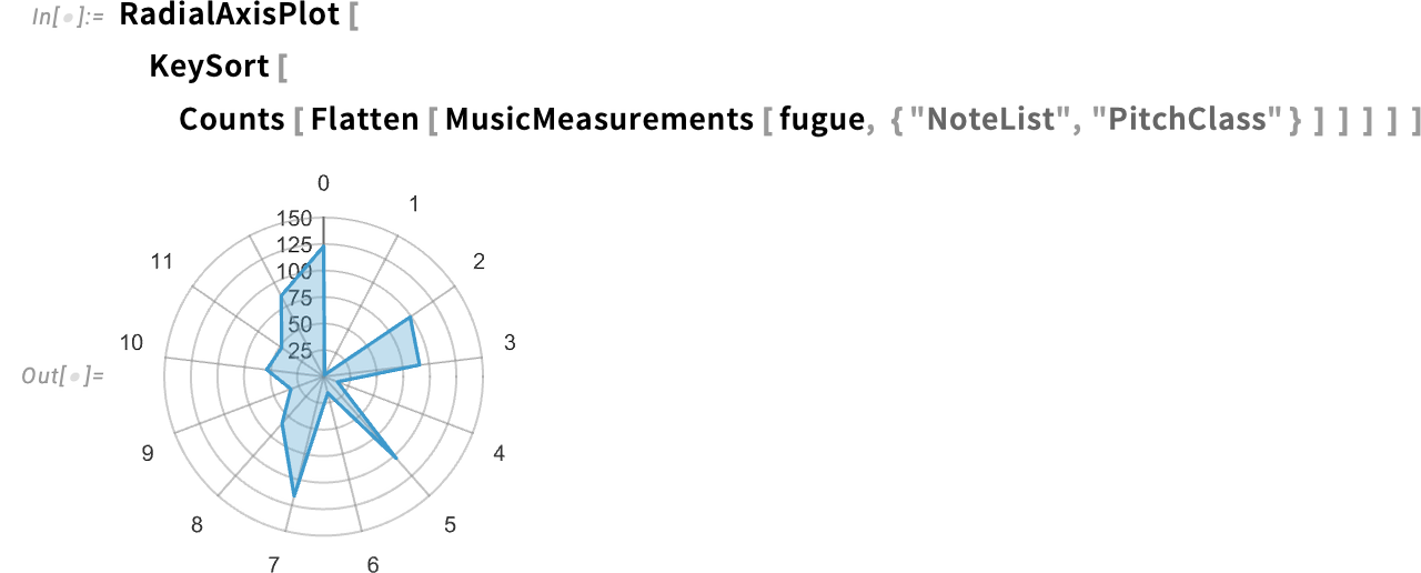
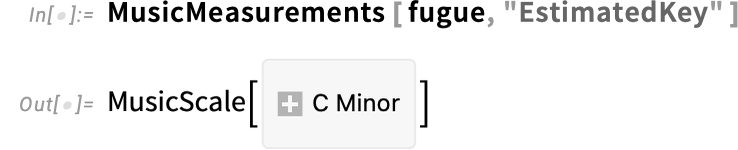
From this plot we can deduce the “effective key” for the score—though MusicMeasurements can do it directly:
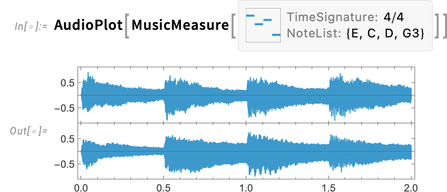
The things we’ve seen here can all be thought of as based on a symbolic representation of music. But given that symbolic representation it’s always possible to render it into actual audio:
Bigger and Better Connectivity for Tabular
The Tabular framework that we introduced in Version 14.2 makes possible extremely efficient handling of tabular data in the Wolfram Language. But where does that data come from? (And, also, where does it go?) In Version 14.2 we introduced highly efficient ways to import CSV etc. files, as well as files in columnar data formats such as Parquet and ArrowIPC. Then in Version 14.3 we added the ability to directly import data from relational databases.
In Version 15 we’re enhancing these capabilities, and adding more. First off, it’s now possible to efficiently import just specific columns from many kinds of files (Version 14.2 already allowed efficiently importing specific rows). So, for example, this imports just two columns from a CSV file:
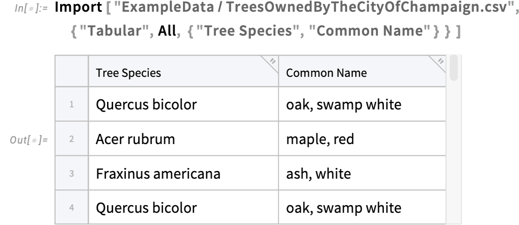
The ability to import only specific columns (and rows) can be critically important in dealing with very large datasets—because it allows you to leave most of the dataset on disk, while efficiently importing into memory just the parts you need.
Where can the original dataset be? It could be in a file on your computer. But DataConnectionObject, introduced in Version 14.2, also provides seamless access to data stores such as Amazon S3, Azure Blob Storage and Dropbox. And now in Version 15.0 we’re also adding seamless access to Azure Files and Azure Tables.
DataConnectionObject also provides access to data in relational databases (something we added in Version 14.3). In Version 15.0 we made this access over an order of magnitude more efficient so that it is now pretty much as fast (and memory efficient) as it can conceivably be.
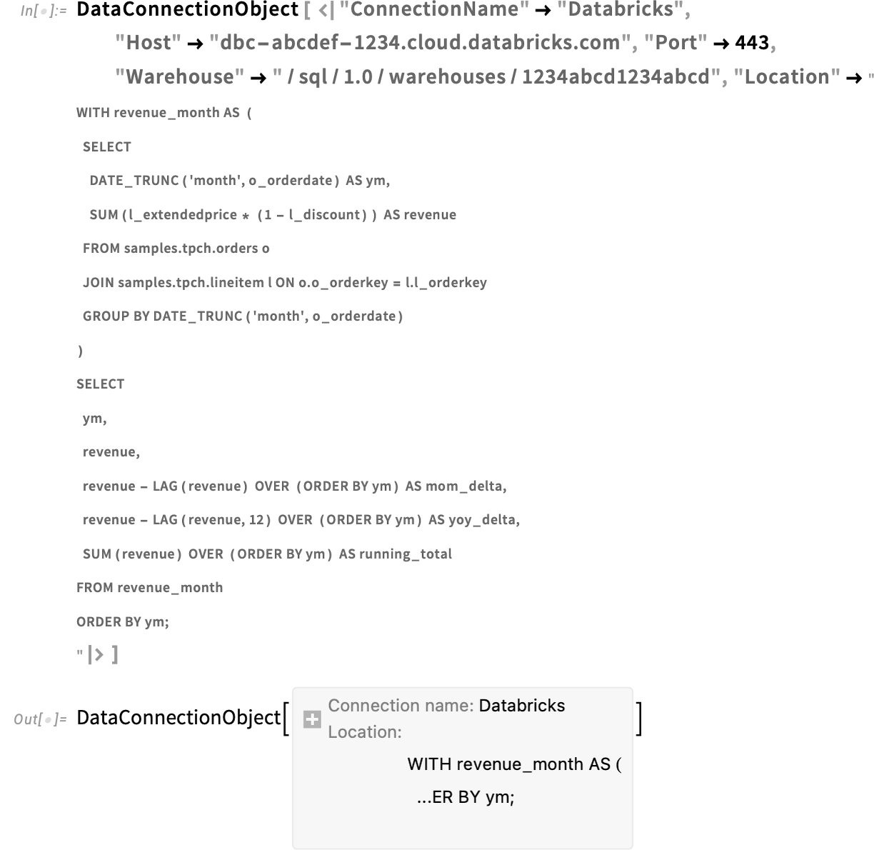
In Version 15.0 we also expanded from relational databases to multidimensional databases, specifically supporting Databricks (as well as Snowflake). So, for example, here’s how one can set up a DataConnectionObject to define a connection to a data “lakehouse” using a particular multidimensional (OLAP) query:
Another new feature in Version 15.0 is the connection of Tabular to ExternalEvaluate, allowing tabular data workflows that include both Wolfram Language and external languages. So, for example, you can get a pandas DataFrame in Python and with ExternalEvaluate immediately get its data in Wolfram Language:
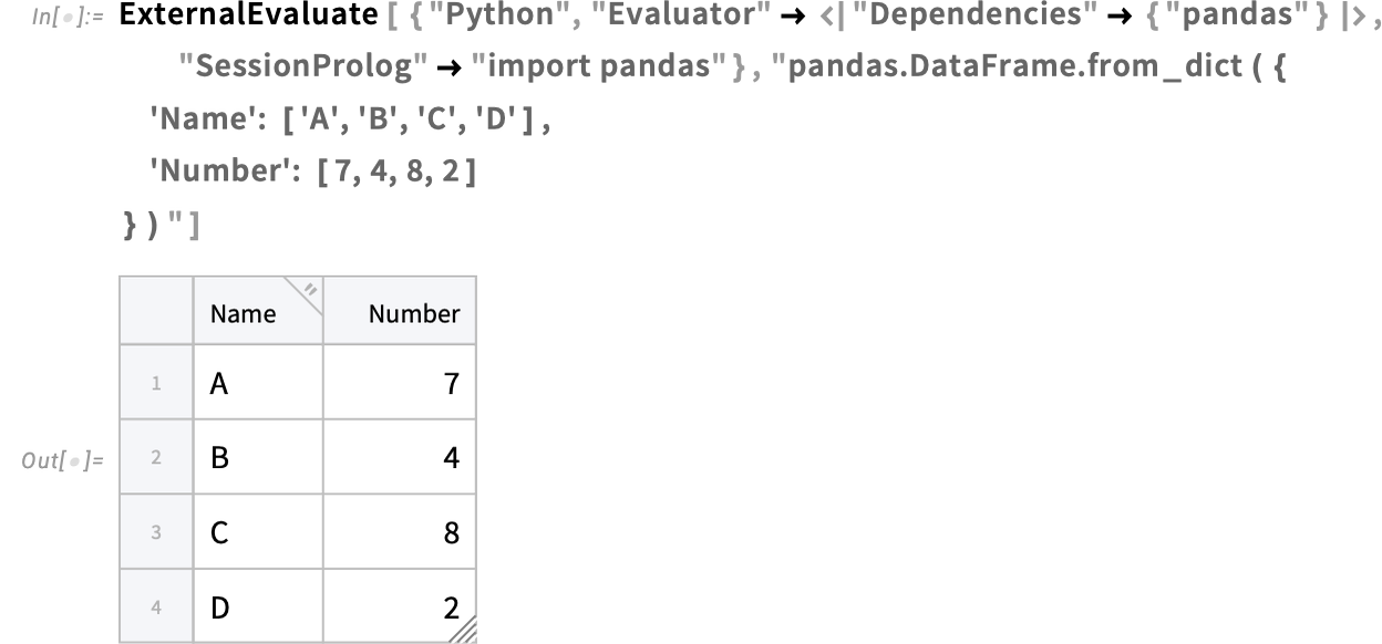
(And, yes, all our work on the encapsulation of languages like Python makes this work in a particularly streamlined way.)
More for Tabular
It took us a long time to develop the original design for the new Tabular framework. And I’m happy to say that the design seems to be working very well. But as is always the case with new frameworks in the Wolfram Language, once the framework is deployed and being used one starts to see all sorts of ways to extend and polish it. And so it is with the Tabular framework. And in Version 15 we’re introducing quite a few enhancements to the Tabular framework.
The first one is simple, but very useful. When you have a fairly small Tabular (say with tens of columns and thousands of rows) in a notebook, all the data “behind” the Tabular is automatically stored right in the notebook, so it’s available whenever you use the notebook. Larger Tabular objects are treated like many kinds of large objects in notebooks (like Video, SparseArray, etc.) and given a button that lets you choose whether you want to store the data directly in the notebook:
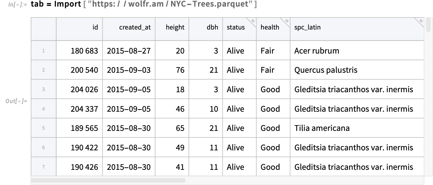
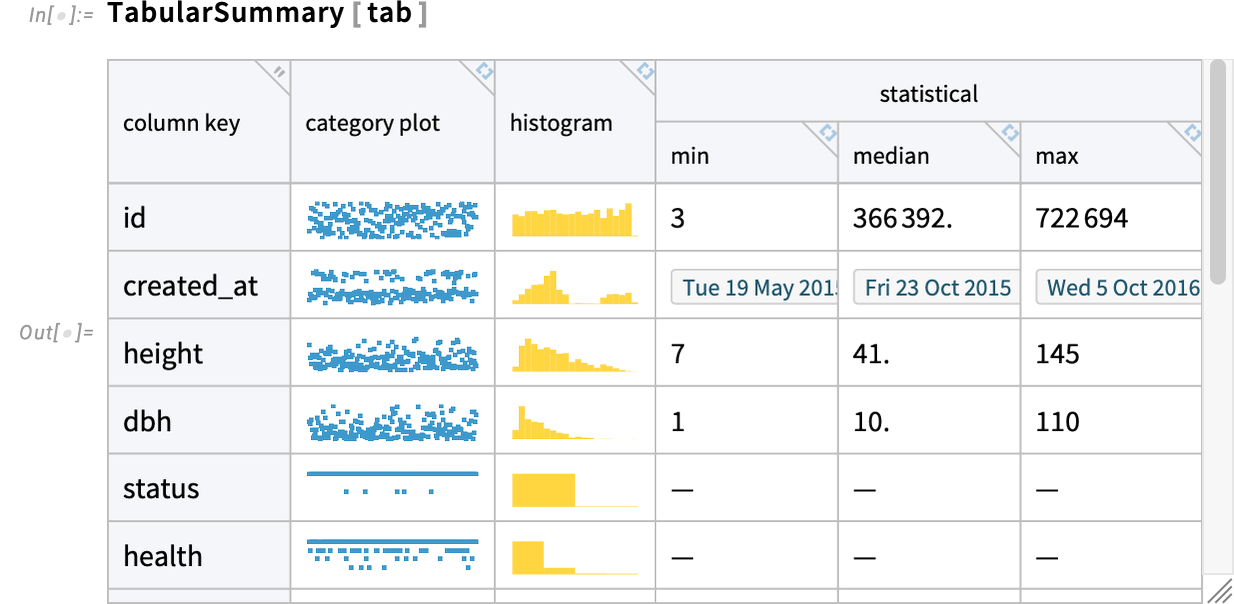
Something else that’s new in Version 15.0 is the function TabularSummary, which efficiently generates an outline summary of Tabular—here the somewhat large Tabular we just imported:
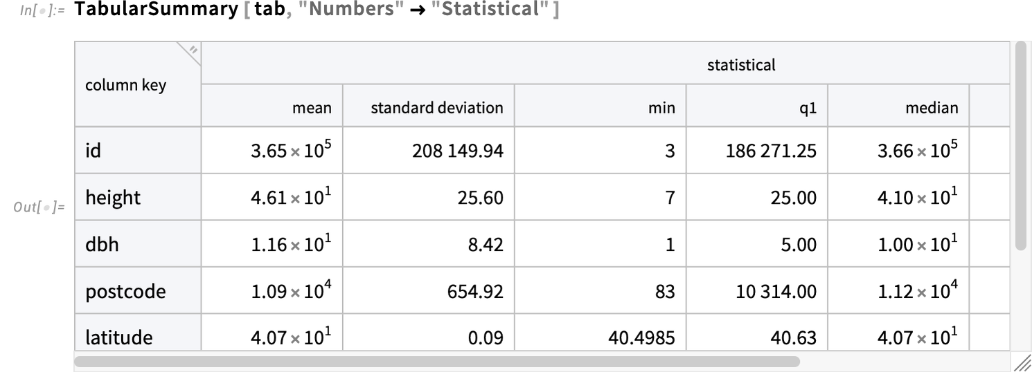
TabularSummary has flexible ways to select what parts of a Tabular to summarize, and how to summarize them. For example, this asks only for columns containing numbers, and asks for a full statistical summary of those columns:
What if we want to model this data? Well, we can immediately use the new Version 15.0 function ModelFit, using the ![]() syntax to pick out particular columns that we can fit a model to:
syntax to pick out particular columns that we can fit a model to:

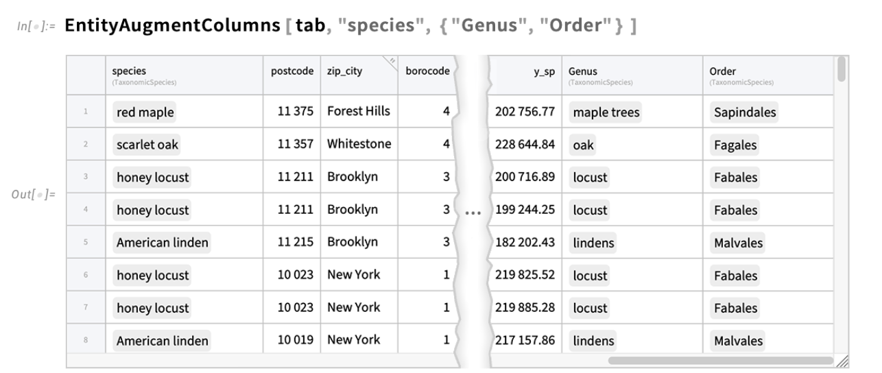
This kind of model fitting works best when we have numbers to work with. But what if your data contains entities—like countries or species of trees? How do we derive numbers from those that we can use to make models? Well, the Wolfram Language contains an immense amount of curated data about all sorts of entities. And in Version 15.0 there’s a new function EntityAugmentColumns that lets you immediately augment a Tabular to add data (numerical or otherwise) associated with entities in a column of the Tabular:
An important aspect of Tabular is that it’s specifically optimized for many common kinds of data, like numbers and dates. In Version 15.0 a new type of data that’s been added is approximate numerical data represented by Around:
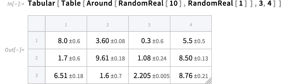
By the way, this example illustrates another new feature in Version 15. We didn’t explicitly name the columns here, so they’re just labeled by numerical indices—which are now given in gray in the display.
There are many other detailed improvements and enhancements to Tabular. One is that GeoPosition columns in Tabular can now handle geo projections, appropriately reprojecting positions when needed.
Visualization Tuneups
Wolfram Language graphics get used in many, many places, and we’re keen to make sure they always have a fresh, lively look. An important part of achieving this has to do with making sure the colors we use “look up to date”. We want our overall color choices to stay consistent. But we also want to periodically “spiff up” colors so they “keep up with the times”.
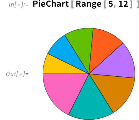
Over the past several versions, we’ve done a lot of spiffing up of colors. Now in Version 15 we’ve turned to the case of regions in charts—like PieChart. So, for example, here’s a pie chart rendered in Version 14.3:
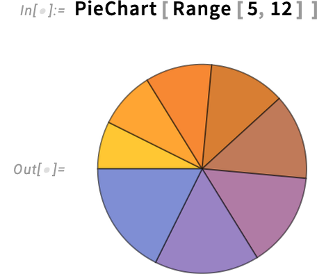
And here’s the spiffed up version for Version 15:
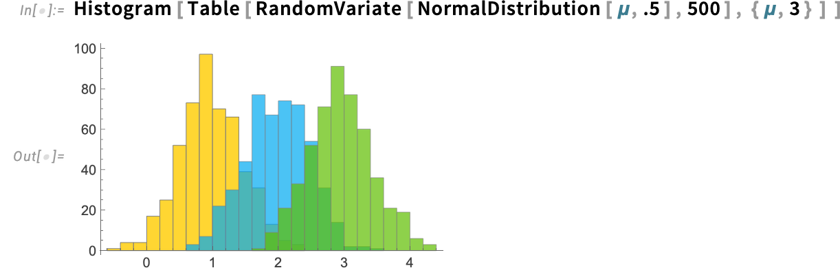
There are also new default colors for things like histograms. It’s a bit more subtle, but
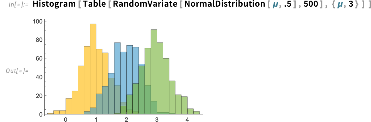
is replaced in Version 15 by:
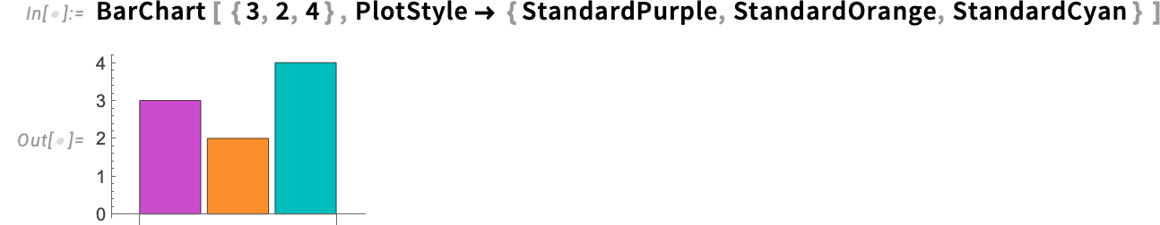
Another new feature in Version 15 has to do with the extension of the PlotStyle option, as well as related options. In previous versions, you’d use PlotStyle to specify styles of curves in Plot, etc., but you’d use ChartStyle to specify styles of bars in BarChart, etc. The reason this distinction was made had to do with handling styles for groups of bars, etc. But in Version 15 we have a more streamlined and unified way to do this—one consequence of which is that we’re able to use PlotStyle for everything, and there’s no potential confusion with sometimes having to use ChartStyle.
So, for example, this now works to style bars in BarChart:
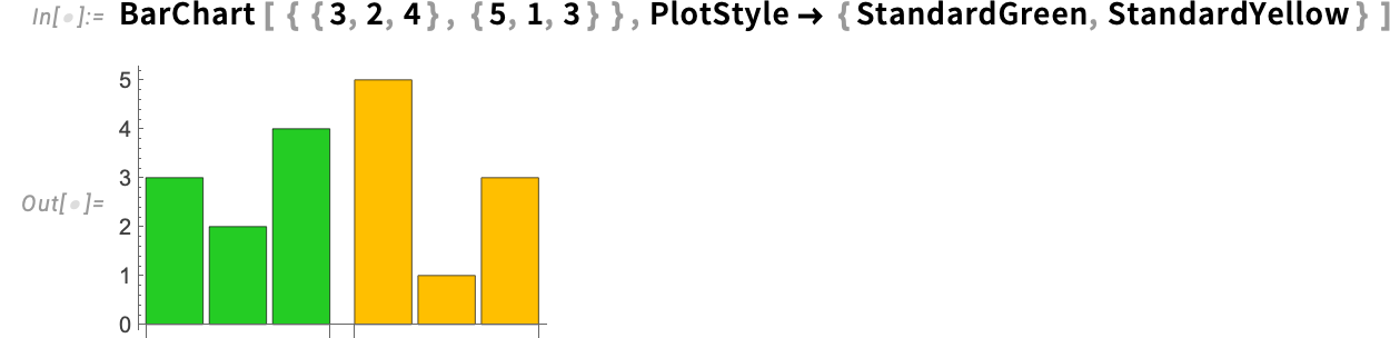
What if you have several groups of bars? ChartStyle by default specifies styles for corresponding bars in each group, but PlotStyle—to be consistent with its use in Plot, etc.—specifies styles for whole groups:
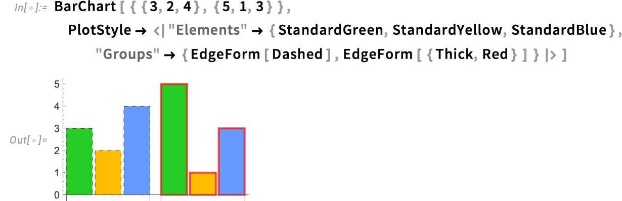
But now, in Version 15, we have a new association-based way of specifying colors, that lets one separately define the styles of “elements” (i.e. individual bars) as compared to groups of bars:
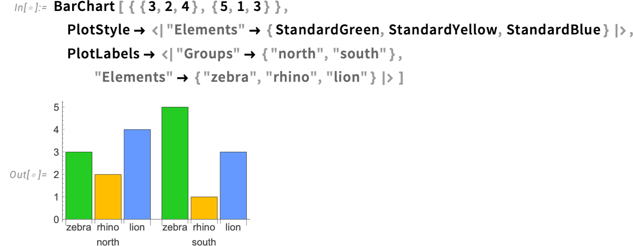
The same association-based mechanism also works for PlotLabels etc.—allowing one, for example, to separately label individual bars versus groups of bars:
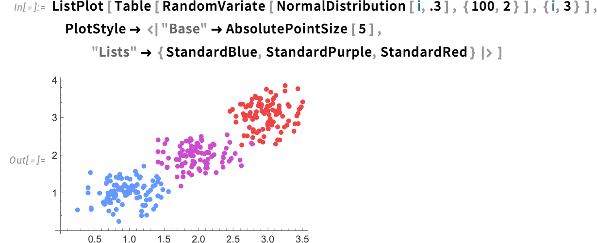
One can also have this kind of detailed control in functions like ListPlot. Here we’re defining a certain “base style”, then saying how different lists of points should be rendered:
Some of what our new association-based mechanism can achieve was already possible with various combinations of existing options. But the association-based mechanism makes it all much clearer and more straightforward.
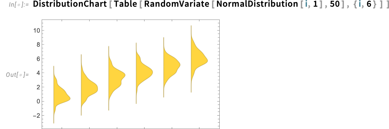
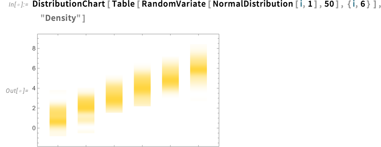
There was a similar issue with DistributionChart; it had great functionality that could only be accessed by slightly obscure combinations of options. In Version 15 we’ve mainstreamed the most important capabilities of DistributionChart (which is, by the way, a very nice and useful function).
Here’s the new default behavior of DistributionChart—visibly generating smooth histogram distributions for each dataset:
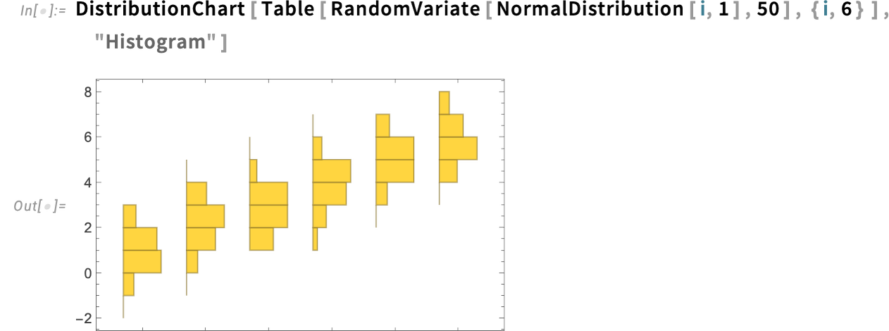
If you don’t want the smoothing, just use "Histogram" as an explicit second argument:
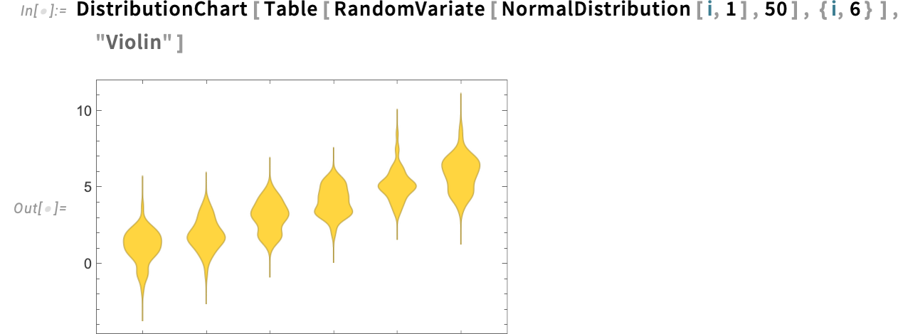
You can get a two-sided “violin-style” appearance if you want:
Or you can just explicitly show density (optionally with quantile lines, etc.):
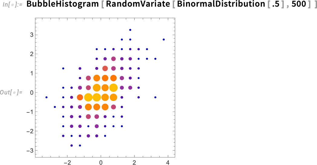
The Wolfram Language has extremely flexible visualization capabilities. But we’re always looking for ways to make more visualizations more convenient. And in Version 15 we’ve added a few entirely new visualization functions to help with this.
One of them is BubbleHistogram. Let’s say you have a collection of {x,y} values. Histogram3D and DensityHistogram are two ways to visualize the distribution of these values. In Version 15 there’s now also BubbleHistogram:
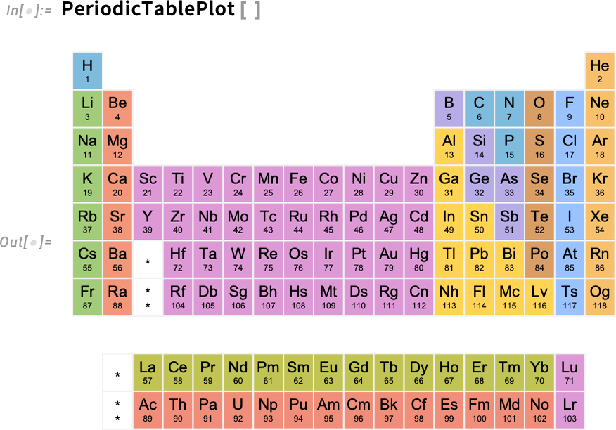
In a completely different direction, Version 15 also adds PeriodTablePlot. If you don’t tell it otherwise, it’ll just “plot a periodic table”:
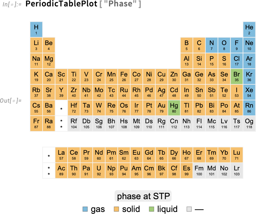
But you can also plot things “over” the periodic table. So, for example, this asks to plot the phase of each element:
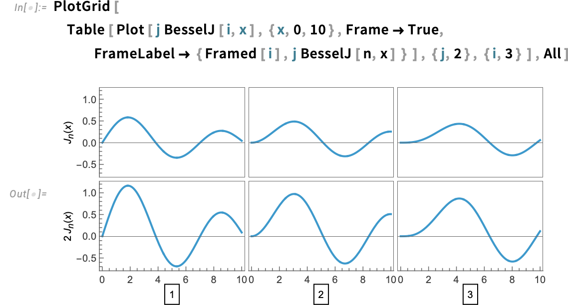
Multipanel Visualization
Let’s say you’ve got an array of plots:
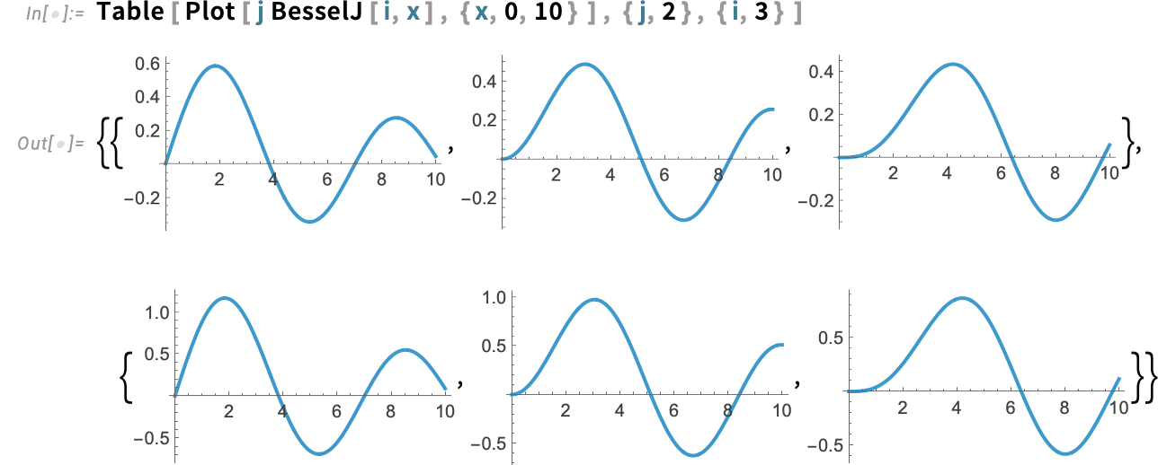
You could display them in a grid:
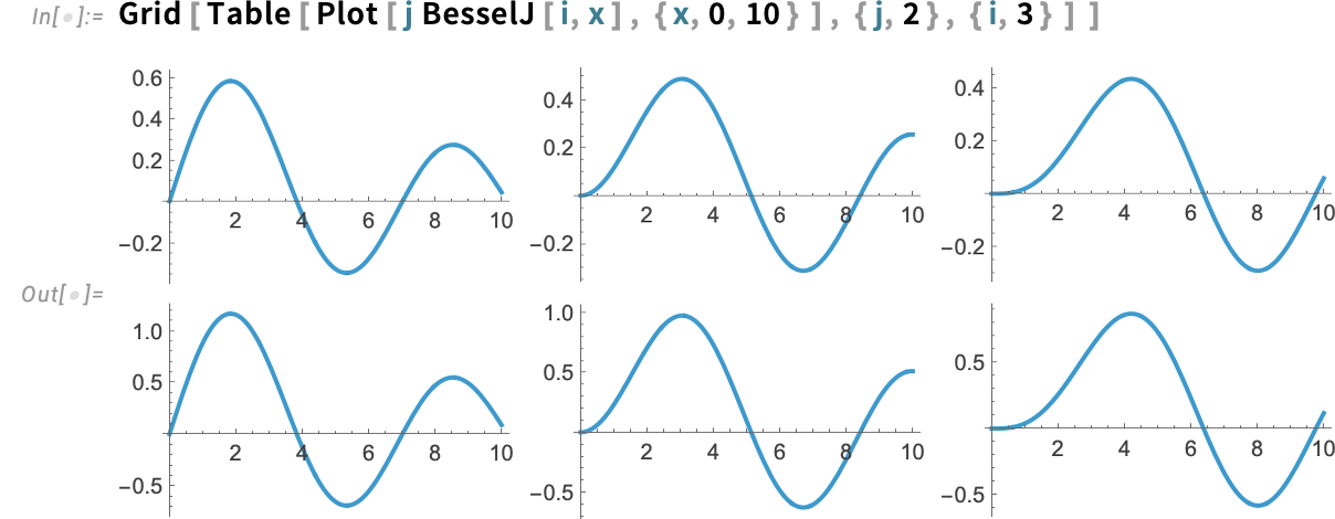
But in a sense this is very wasteful (and “noisy”): the plots basically have the same scales, but we’re repeating these scales for each plot. In Version 15 we now have a new function, PlotGrid, that takes a collection of plots and tries to optimally render them in a grid, sharing as much scale information as possible:
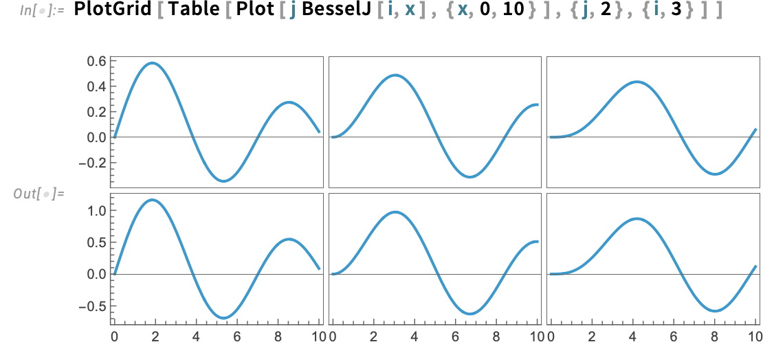
There are many subtleties to this. One that’s visible in this case has to do with whether scales are shared between different rows and different columns, or merely within each row and each column.
Here’s how you ask for all scales to be shared—in this case now making the y scales on the two rows the same:
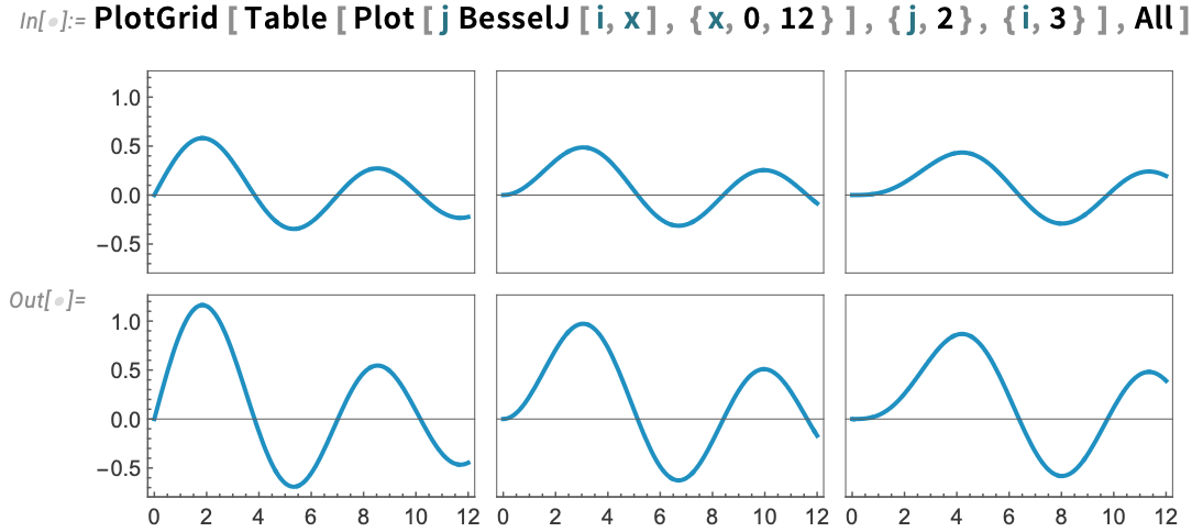
PlotGrid also handles labels, again by default sharing them where it can:
In effect, PlotGrid “harvests” options from the individual plots, then tries to combine them to make a consistent overall grid. PlotGrid itself can also be given options. For example, you can specify overall AspectRatio or ImageSize in PlotGrid. But you can also give ItemAspectRatio and ItemSize options to PlotGrid, that specify the aspect ratio or size of each individual item in the grid.
Gigabyte-Sized Notebooks and Real-Time Find
We first introduced notebooks with Mathematica 1.0 in 1988. And I think it’s fair to say they’ve been a great success, both as a way to do work, and as a way to present and remember what one’s done. Back when we first introduced notebooks, the concept that they’d be more than a few megabytes in size seemed inconceivable. But—four decades later—notebooks can be very big. Sometimes it’s because they contain large graphics. Sometimes it’s because they have large iconized expressions. And sometimes it’s because someone hit Save in Notebook to save a video or a large tabular dataset right in the notebook.
We’ve done quite well in many ways at handling large notebooks. But often in the past we needed to make tradeoffs to handle the comparatively small memory and slow mass storage of typical computers. But as the sizes of the largest notebooks started to approach gigabytes, we realized that we needed new notebook infrastructure. So, nearly a decade ago, we embarked on a large project to rebuild our notebook infrastructure from the ground up. Well, I’m excited to say that that project is now finished—and Version 15 has all-new highly efficient multicore multithreaded notebook infrastructure.
The result is that one can now routinely deal with multi-gigabyte notebooks (and there’s nothing other than storage that ultimately limits the possible size of notebooks). In all of this, we’ve maintained complete compatibility—so Version 15 can still open notebooks that were created in Version 1 (and, yes, we tested that very extensively). The underlying structure of notebook files is still the same as it ever was. But what’s allowed us to achieve the kind of performance we have in our new notebook infrastructure is a complete rethink of the way we parse notebook files, making use of modern multi-pass parsing methods.
But with the routine use of huge notebooks come new issues. Notable among them is Find. And in Version 15, building on our new notebook infrastructure, we have an all-new highly-efficient Find system.
Press CMDF/CTRLF in a notebook and you’ll get a Find dialog for that notebook:
![]()
Things are so fast that as soon as you start typing you’ll see a tally of how many matches there are in the notebook. (And that works even if the notebook is gigabytes in size.)
The Find dialog mostly works in a very standard way. Each match in the notebook is highlighted. ![]() (or ENTER) goes to the next match—and the nnn/nnn display in the input field shows which match you’re at.
(or ENTER) goes to the next match—and the nnn/nnn display in the input field shows which match you’re at. ![]() is a toggle for case sensitivity, and
is a toggle for case sensitivity, and ![]() for matching whole words.
for matching whole words.
Press > and you open the replace part of the Find dialog:

Press ![]() to do one replacement, and go to the next one. Press
to do one replacement, and go to the next one. Press ![]() to do them all.
to do them all.
There are lots of details to how Find needs to work in Wolfram Notebooks. One is handling typeset expressions and special characters. And indeed you can enter a typeset structure and find it:
![]()
Special characters, like α, work too. Though you can’t use ESC to enter them, because at a system level this dismisses the Find dialog. You can still use long names such as \[Alpha], as well as SHIFTESC.
There’s another subtlety as well. In doing replacements, you only want to replace “input” material in the notebook; you want to skip material that appears in generated output. And this gets indicated by the fact that things you find in generated output have a dashed border in their highlights:

Ever since we introduced them in 1988 notebooks have fundamentally been “single-pane” documents, primarily intended to maintain a linear sequence of sometimes-dynamic content. And when another pane is needed, the typical pattern has been that it should be another notebook. In the Wolfram Cloud—following typical patterns on the web where everything ultimately has to fit in one browser window—we have nevertheless had various kinds of sidebars for many years. Well, now sidebars are also coming to desktop notebooks. In future versions, there’ll be quite general mechanisms for sidebars. But in Version 15 sidebars are being introduced for two specific, high value purposes: notebook properties, and the AI Assistant.
In any notebook, click the gear icon in the toolbar (or choose from the Window > Sidebars menu) and a notebook will sprout a Notebook Properties sidebar that allows you to see (and modify) various commonly used notebook-level settings:

Another application of sidebars in Version 15 is for the AI Assistant. The chatbar lets you create chat cells in your main notebook window. But sometimes it’s convenient to have a “side chat” with the AI, that doesn’t directly affect the main content of your notebook. The ![]() button in the notebook toolbar opens a side chat—in a sidebar:
button in the notebook toolbar opens a side chat—in a sidebar:

(You can adjust the width of the sidebar just by dragging the divider in the window.)
Visual Themes Come to Notebooks
Not everybody wants their notebooks to look the same. And being able to switch between light and dark mode is one major way different people can see even the same notebook very differently. But in Version 15 there’s another major way to make a notebook look different: change its visual themes. You might want to do this to emphasize syntax coloring more, or less. You might want to do it for accessibility, or just as an aesthetic preference.
You can change notebook themes either for specific notebooks, using the Notebook Properties sidebar, or globally for all notebooks, using the Preferences panel. (You can also change notebook themes programmatically, by setting the NotebookTheme option.)
Here’s the Theming section of the Preferences panel (that includes both standard modern themes like Monokai, Solarized and Dracula, as well as themes we’ve designed like Wolfram Saturated and Stargazer):

Choose any theme, and it’ll immediately be applied to your notebooks. Note that for each theme, there’s both a light mode and dark mode version.
If you set a theme in global preferences, it’ll just be used to determine the look of notebooks on your system; if you send a notebook from your system to someone else, it’ll be their themes, not yours, that determine how it looks to them. But if you set a theme for a specific notebook using the Notebook Properties sidebar then that theme will be carried along with the notebook, and anyone you send the notebook to will see it.
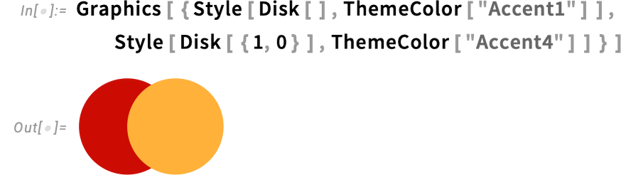
Notebook themes are actually based on a feature introduced in Version 14.2: ThemeColor. The way notebook themes work is that different elements of a notebook are tagged as being rendered in different named colors. For example, title cells in the default stylesheet are tagged as being rendered with named color "Accent1":
As another example, entities are rendered with "Accent4":
Let’s say you want to match these colors in a graphic. Well, you can do that by referring to these named colors:
If someone switches their theme to, for example, CRT, then this will immediately look different for them:

With the introduction of visual themes for notebooks, another new feature in Version 15 is an extension to the color picker to allow selection of named colors:

When It’s Too Long, It’s Torn Off
Let’s say that—like I often do—you’re using notebooks as a medium of exposition. What should you do with long pieces of output? If you leave them in an open cell in the notebook they break the flow of your exposition. But if you close the cell, nobody can tell anything about what was in them. Well, in Version 15 there’s another alternative: just tear it off.
Select the cell and choose Cell > Elide with Tear in the main menu (or in the right-click menu):
Once you’ve got the tear, you can just drag it up and down:
It’s all rather simple—but very useful. And, actually, I’ve been using this mechanism for years in things I’ve written (including about previous Wolfram Language releases!) There’s been a function in the Wolfram Function Repository to do a standalone (and parametrized) version of it for a couple of years. But now in Version 15 it’s fully integrated into our notebook system.
How does it actually work? Well, the “tear” is generated from a deterministic random process seeded by the UUID assigned to the cell—so the tear will always look the same in that particular cell, but will be different if, for example, you copy the cell. (The actual rendering of the tear is done using an efficient pixel shader.)
By the way, you can add a tear to absolutely any cell—whether it contains an image, text, interactive content, etc.:
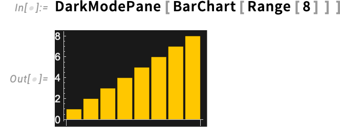
Going Dark in the Light
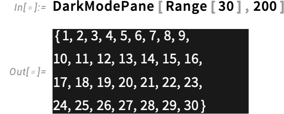
Let’s say you’re working in light mode in a notebook, but you want to get one picture in dark mode (say for a presentation). In Version 15 there’s an easy way to do this: just use DarkModePane:
There are the same options here as in Pane:
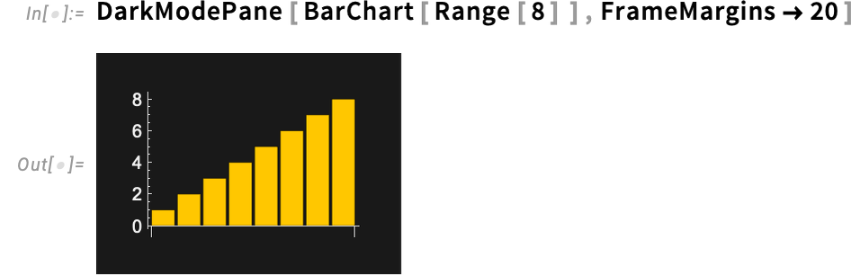
You can specify a wrapping width:
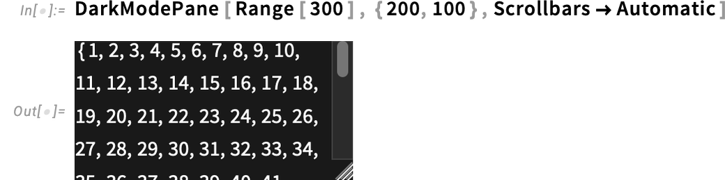
And a height—with scrollbars optional:
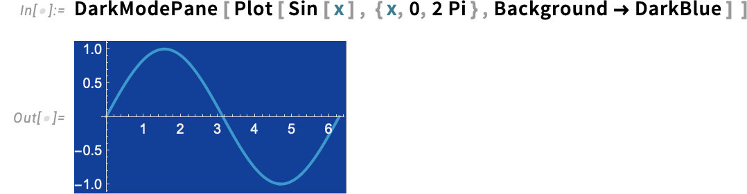
And, yes, if you’re in dark mode, you can do the exact opposite of all this, using LightModePane. Oh, and if you want to use some special, dark color as a background for your output, DarkModePane is a good way to “flip” everything (like axes and their labels) to dark mode:
By the way, if you’re documenting what happens in light and dark mode, you’ll need LightModePane and DarkModePane—and these will be showing up a fair amount in our documentation.
What’s Happening in that Computation? The One-Argument Form of Monitor
How do you tell what’s happening inside a computation you’re doing? You could insert some Echos. Or—ever since Version 6—you could use Monitor. But the way Monitor has always worked in the past, you’ve needed to explicitly tell it the variables whose values you want to monitor. And that’s been fine for monitoring functions like Table, where there are named variables to deal with. But what about something like Map? How can you monitor that?
Well, in Version 15 there’s a new, one-argument form of Monitor, that lets you monitor a function like Map:
The blue box that pops up shows you how far the Map has got, as well as an estimate of how much longer it should take to finish. (It also includes a ![]() button to abort the computation.)
button to abort the computation.)
The one-argument form of Monitor works with all the obvious functions—like Map-related ones, Nest– and Fold– related ones, Table-related ones, etc.
For something like Table, you can always use the two-argument form, specifying what you want to monitor:
But the one-argument form just “does it all”, giving you information on overall progress, without you having to explicitly think about individual iteration variables, etc.:
The two-argument form Monitor[expr, mon] will monitor all changes in the value of mon that occur during the evaluation of expr. Monitor[expr], on the other hand, only looks at the evaluation of the top-level function in expr. In other words, in its one-argument form, Monitor needs to be wrapped directly around the function you want to monitor, whether that be Map, Fold, Array or whatever.
Subvalues Can Now Be Held!
It’s a corner case that for nearly forty years we imagined one day we’d handle, but it always seemed hard. Well now in Version 15 we finally did it: subvalues can now be held!
What does this mean? First, what’s a subvalue? When you make an assignment like
you’re making an assignment for what we call a downvalue of f. But what if you make an assignment like:
In that case we say you’re assigning a subvalue for g.
Subvalues are useful for many purposes, particularly in setting up operator forms like:
OK, so what about the concept of holding? Normally, if you enter f[1+1] what happens is that first
Why is this useful? Imagine saying x = 1, which is interpreted as Set[x, 1]. It’s important that the x here is held. You want to set the value of “x itself”, not the value of x. So you need to pass x to Set without it being evaluated first.
The fact that things work this way is determined by the attributes of Set: the HoldFirst means that the first argument of Set should be held:
Let’s say you make the assignment:
Now the first argument of u will be held—though others will not:
Meanwhile, if you make the assignment
all arguments will be held:
Alright, so what’s the interaction between holding of arguments and subvalues? Let’s say you have an expression like u[x][y]. If u has attribute HoldAll, then in something like u[x][y] the x will be held—but the y won’t be:
Well, now, in Version 15 there’s a new attribute SubValuesHoldAll—which holds all subvalue arguments. Set this attribute
and now in v[x][y] the y gets held, even though the x is evaluated:
And, by the way, the holding “goes all the way down”:
Why is this useful? Most importantly because it allows one to have operator forms which hold their arguments. In designing all sorts of functions, we’ve wanted this for years. Consider, for example, AppendTo. AppendTo has attribute HoldFirst, so that AppendTo[x, expr] (like Set[x, expr]) doesn’t evaluate x.
But what about an operator form of AppendTo? We’d like to be able to say AppendTo[expr][x] and have this append expr to x. But to do that requires that x be maintained unevaluated. Which—thanks for SubValuesHoldAll in Version 15—is now possible.
Operator forms make for particularly elegant and convenient functional programming. And especially in the past decade or so, we’ve increasingly been introducing such forms for a wide range of functions. But for some functions (like AppendTo) we haven’t been able to do this—because we haven’t had SubValuesHoldAll. And, yes, in terms of internal implementation SubValuesHoldAll is tricky—because it involves a kind of “evaluation lookahead” that has to be handled very carefully. But now in Version 15 it’s done, and we can open the design opportunities for lots of new and useful operator functions, as well as other uses of subvalues.
Introducing Ready-to-Use Incremental Data Structures
Let’s say you want to search through a billion objects, perhaps picking out ones with some special property. What would potentially make for the cleanest code is just to generate the billion objects, then pick out the ones you want. But of course the billion objects might be hard to store in memory. And you might imagine that the only way to handle this would be to figure out how to generate the objects sequentially, then write code that explicitly loops over the objects.
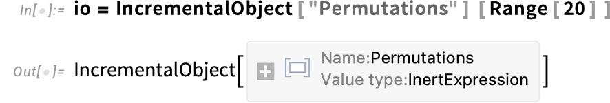
Well, in Version 15.0 there’s a better, cleaner—and more efficient—way to do this, using our new IncrementalObject construct. IncrementalObject is is based on the IncrementalFunction technology we introduced in Version 14.3, but now it’s packaged for immediate use, and doesn’t require explicit code compilation, etc.
The basic idea of IncrementalObject is to provide a symbolic representation for a (potentially very large) collection of things, set up so that the things can be incrementally accessed. So, for example, this incremental object represents the 20! ≈ 2 x 10¹⁸ permutations of 20 objects:
Every time you ask for NextValue of this incremental object, you’ll now get the next permutation in the sequence:
So now let’s say you want to find the first permutation that has order 20. You can use the incremental version of Select:
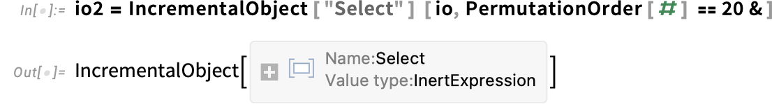
The IncrementalObject you get here is just a symbolic representation of the selected permutations. If you want to actually find the first permutation in this selection, you can do that using NextValue:
Run NextValue again to get the next permutation in the selected set:
And, yes, it has order 20:
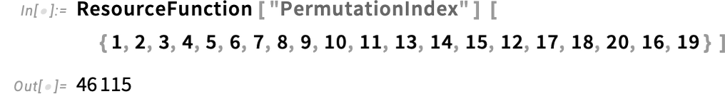
In case you’re wondering, here’s how many permutations had to be tested to get to this one:
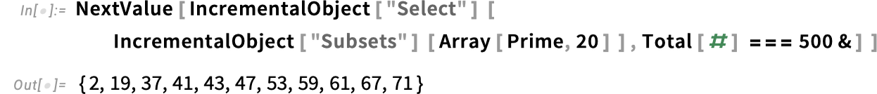
Here’s another example, this time using the incremental version of Subsets, and solving the knapsack-style problem of finding a subset of the first 20 primes that add up to 500:
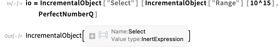
In Version 15.0 we have incremental versions for a variety of functions. Beyond Permutations and Subsets, there’s Tuples, and there’s Map, FoldList, Take, and Range. Here’s an example using Range, searching for perfect numbers:
What if we want to go further? Maybe we’d like to do the computation on a different computer. Well, we can just pick up the IncrementalObject we got here, and start running it again on another computer. It’s a (transportable) symbolic expression that represents (“lazily”) the current state of our computation, ready to be continued at any point.
There’ll be more coming with incremental computation in future versions. But IncrementalObject already provides a convenient new way of organizing computations, allowing one to think in an “enumerate first, select later” way, but with the computation automatically implemented sequentially with very small use of memory.
Exceptions and Error Handling in Large Codebases
When one writes a program one presumably has in mind what it should do. But what if something goes wrong? In effect there need to be secondary code paths that sensibly handle whatever errors can occur. And in larger codebases the issue of handling errors in a sensible and organized way tends to become more and more important.
In Wolfram Language we’ve had a variety of ways of dealing with errors ever since Version 1. And they typically work well at a local level within particular functions or modules. But in Version 15 we’re now introducing a powerful new global mechanism for handling errors, using the concept of symbolic exceptions.
Before we get into that, let’s recap the existing Wolfram Language mechanisms for handling errors.
At a very minimal level, there’s the idea that under certain circumstances a particular function just won’t be evaluated (like if a pattern doesn’t match, or a /; condition isn’t satisfied), and will “return its symbolic unevaluated form”. Then there’s the idea of explicitly using Return to exit a function if something goes wrong.
But both these mechanisms are very local; they handle errors only within a single function.
Well, even in Version 1 there was already a mechanism—which has been widely used ever since—for nonlocal error handling: Throw and Catch. Call Throw anywhere in your code, and it will stop what it’s doing, and return to the nearest enclosing Catch. But here’s the catch (so to speak): what if somewhere in functions you are calling (that perhaps you didn’t even write yourself), there’s a Throw? If the code hits that Throw, it will throw off (so to speak) everything your code is doing.
The general mechanism of Throw and Catch is a powerful way to handle errors. But the challenge is to control and scope it properly. In Version 3 (1996) we introduced tags for Throw and Catch, which provide a good basic low-level mechanism for scoping Throw and Catch. But in practice, particularly for larger codebases, they’re fiddly to use and difficult to manage.
Many years went by. But finally in Version 12.2 (2020) we introduced another, very clean mechanism for handling fairly local errors: Confirm and Enclose. The idea is to have Confirm-family functions (Confirm, ConfirmQuiet, ConfirmBy, ConfirmMatch, …) sprinkled inside a piece of code which don’t affect the operation of the code assuming that they correctly confirm whatever they’re being asked to confirm—but if something goes wrong, they stop the code, and return to the nearest enclosing Enclose. In their most common form, Confirm and Enclose directly appear inside a single function, and are handled lexically, without the need for any explicit tagging. This is extremely convenient for dealing with errors within one function, but if one wants to propagate errors beyond that function it requires explicitly requesting that propagation at each level using additional instances of Confirm and Enclose.
So what can one do if one has a large codebase in which errors can occur in one function, and need to propagate out, potentially through many other functions that know nothing about that error? Well, in Version 15 we’re introducing a mechanism for dealing with this, using symbolic exceptions.
The basic idea is quite simple: use ThrowException to throw a named exception that will propagate up to the nearest enclosing CatchExceptions that is set up to handle exceptions of the relevant type. Typically the names of exceptions are symbols, which can be scoped in packages using standard scoping mechanisms, including the new ones we’re introducing in Version 15. Importantly, there can also be a hierarchy of types of exception, so that a CatchExceptions for a more general type of exception can catch any subtypes of exceptions that occur within it.
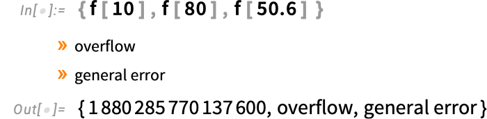
As a simple example, let’s define a function fac that can throw an exception:
Now let’s define a function g that uses fac
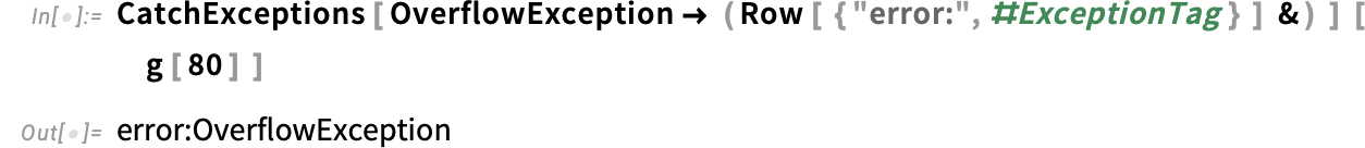
and then another function f that uses g, but now catches the overflow exception:
Now we can use f, and if no exception is generated, it just computes its value as usual:
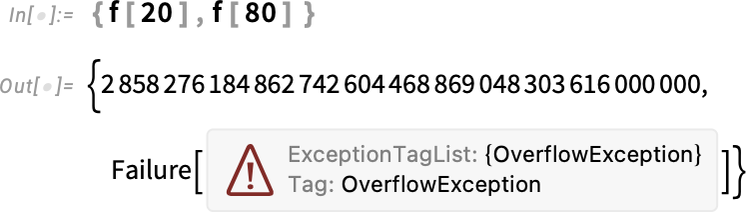
But if there is an exception generated anywhere inside the evaluation of f, it’ll propagate up, and the value of f will be (by default) a Failure object:
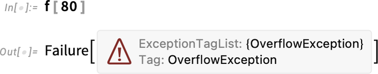
Note that because f catches the exception, any error doesn’t propagate beyond the evaluation of f:
But what happens if we evaluate g directly? Then there’s no CatchExceptions to catch any exceptions that are generated, and so the exception “takes over everything”:
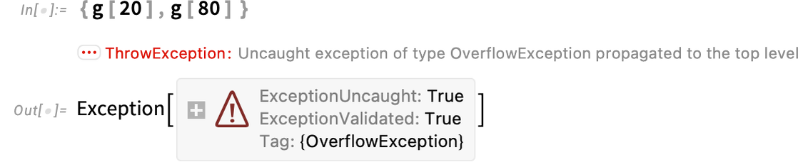
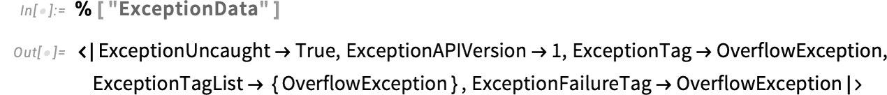
What gets returned in this case is the underlying Exception object: a symbolic representation of the exception that was generated. Exception objects contain several pieces of data:
CatchExceptions can use this data. Here we’re saying that if we are dealing with an exception of type OverflowException, then we should return the result of applying the specified function to the Exception object:
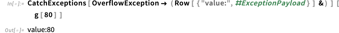
It’s often convenient to give an explicit “exception payload” when the exception is thrown. Here we’re redefining fac to include x as a payload if it generates an exception:
Now our CatchExceptions can make use of the payload:
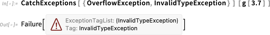
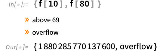
OK, so what happens if we have multiple types of exceptions? For example, let’s say we introduce an InvalidTypeException in fac:
In principle, we can catch both of these exceptions by specifying their types in a list for CatchExceptions:
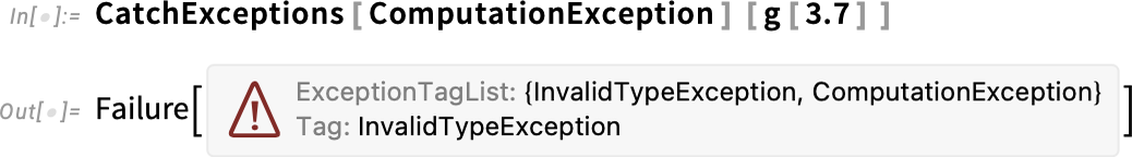
But particularly when you’re dealing with lots of types of exceptions, it’s much more convenient to define a hierarchy of exceptions. You can do this using the function RegisterExceptionType. Here we’re registering both OverflowException and InvalidTypeException as subtypes of ComputationException:
Now we only need to use ComputationException to catch either OverflowException or InvalidTypeException:
We can also set up more nuanced handling of exceptions, in which we give different actions to perform when different exceptions occur:

In our definitions here, we’ve used an explicit If to determine whether to throw an exception. But in writing easy-to-read code it’s often better to use Confirm-family functions than explicit conditionals. And our new exceptions framework interoperates seamlessly with the existing tagging mechanism in Confirm and Enclose. So here’s our fac function written using ConfirmBy:
The CatchExceptions in f will now catch the OverflowException produced by ConfirmBy—and we see two messages: one from the ConfirmBy and one from the CatchExceptions:
The exceptions framework in Version 15 is a powerful one, that makes it easy to add good error handling to large codebases. And in fact, we’ve been using preliminary versions of the framework for several years in the development of internal code for Wolfram Language. What’s in Version 15 represents the major part of what’s needed for large-scale exception handling. There are some additional features to come, notably error translation, in which an error generated in one piece of code can be translated to be appropriate for another piece. (For example, a specific internal overflow error might be translated to a more general “that function can’t be computed” error.) Related to this, we’re also planning to introduce an ontology of errors generated within built-in Wolfram Language functions, that error handling in code written in Wolfram Language can make use of.
Introducing the Structured Package Format
What x is that x? Does the x that appears in one piece of code refer to the same symbol as the x in another piece of code? Within a single piece of code, one can localize a name (like x) using Module. Across different pieces of code, ever since Version 1.0, one’s been able to distinguish different instances of a name (like x) using contexts. one`x is a different x than two`x. Of course, it would be inconvenient to have to explicitly specify a context (like one`) for every instance x. So (again since Version 1.0) there’s been a notion of a current context $Context that allows one to specify in what context any new symbol (say x) will be created, and the notion of $ContextPath that gives a list of contexts to search for a symbol (say x) that’s given in input. Having $Context and $ContextPath helps in avoiding having to explicitly specify contexts all the time. But they’re not enough. And (again since Version 1.0) there’ve been the functions BeginPackage, Begin, End and EndPackage that manage setting $Context and $ContextPath.
And so it’s been (ever since Version 1.0) that Wolfram Language packages have contained incantations of BeginPackage, etc. But there’s always been some messiness to this. Yes, symbols within one package can be localized. And a package can have subpackages. But it’s always been complicated to have symbols that are, for example, localized but shared between packages. Over the years, a variety of different mechanisms for this have been invented. But within our company we’ve slowly converged on one particular mechanism. And now in Version 15.0 we’ve built this mechanism into the Wolfram Language as the new Structured Package Format.
The Structured Package Format is particularly important when one’s dealing with larger amounts of Wolfram Language code—and specifically code that is spread across multiple files in a directory tree. In our traditional package setup, there’s no particular significance assigned to what file a symbol is defined in. But in the Structured Package Format the crucial assumption that’s made is that symbols defined in different files are by default different, in the sense that their names are taken to be in different contexts. In other words, in the Structured Package Format, new symbols are by default “born private” (i.e. localized) within their files.
But what if one wants a particular symbol x to be “public”, and available outside its file? Then one can declare a symbol to be exported using PackageExported. So in Structured Package Format it’s typical for a file to contain something like:
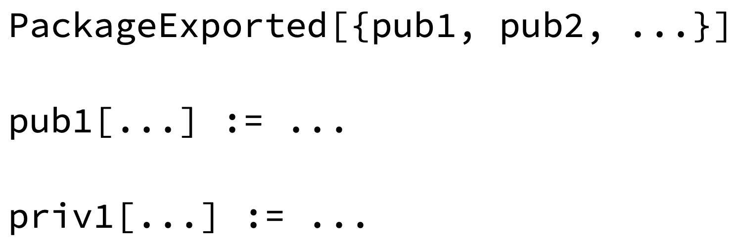
The functions pub1, etc. are exported to be public functions, while priv1, etc. are kept localized as private functions within the file. And if you want a symbol to be shared between different files in a package, but not to be accessible outside the package, all you need do is put it in PackageScoped rather than PackageExported.
So how does one set up a whole package in Structured Package Format? Well, you put its files in a directory tree. And—at least in the simplest case—at the top level of that directory tree you have a file init.wl which contains PackageInitialize[“name“], where (normally) name is both the name of the base context for your package, and the name of the top-level directory for the package. (When the package is part of a paclet, the PacletInfo.wl file for the paclet can specify more elaborate directory structures, different initialization file names, etc.)
When you use a package in Structured Package Format, you call Needs with a context name just as you would for a traditional Wolfram Language package—and this loads the init.wl file in the corresponding directory. And it’s when PackageInitialize is run that the magic of the new Structured Package Format happens—and the other files in the directory tree are loaded, with their symbols by default localized.
There’s one last function in Structured Package Format to mention: PackageImport. When PackageInitialize is loading files, you sometimes want to import definitions from other packages. PackageImport lets you import either all public symbols from a given package, or, importantly, just particular public symbols you need from that package.
In the traditional (since Version 1.0) way of setting up packages, you end up with BeginPackage, Begin, etc. strewn through your code. The new Structured Package Format lets you avoid all that, and specify what symbols should be accessible where in a very clean and minimal way.
Why did it take us all these years to come up with this? To a user, the Structured Package Format seems pretty simple in its operation. But what’s happening underneath is quite elaborate. Here’s one of the issues. If PackageInitialize encounters an x in a file of Wolfram Language code, it has to know in what context that symbol x is supposed to be. But that’s potentially only defined by what appears later in that file, or in some quite different file. So how does PackageInitialize deal with this? Well, it first scans the whole directory tree, harvesting all instances of PackageExported and PackageScoped, and only once it’s processed these and determined the contexts for symbols does it actually read the full code in the directory tree. In other words, there’s an essentially lexical pass done on all files before the “real” semantic pass. And, yes, it’s very tricky to have this all work in all cases. But in the new Structured Package Format it does—and it allows one to set up large Wolfram Language codebases in a better and cleaner way than ever before.
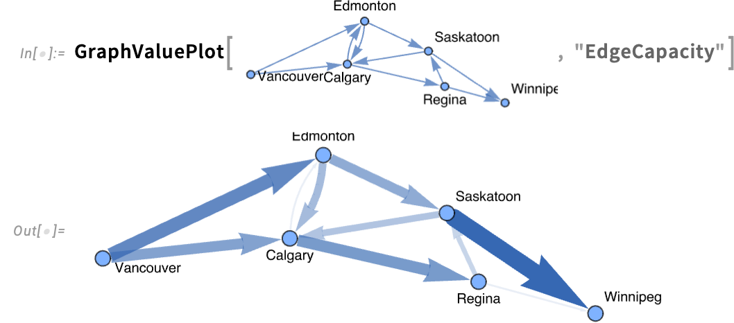
Plotting over Graphs
How do you plot values on the nodes of a graph? In Version 15 you can just use GraphValuePlot:
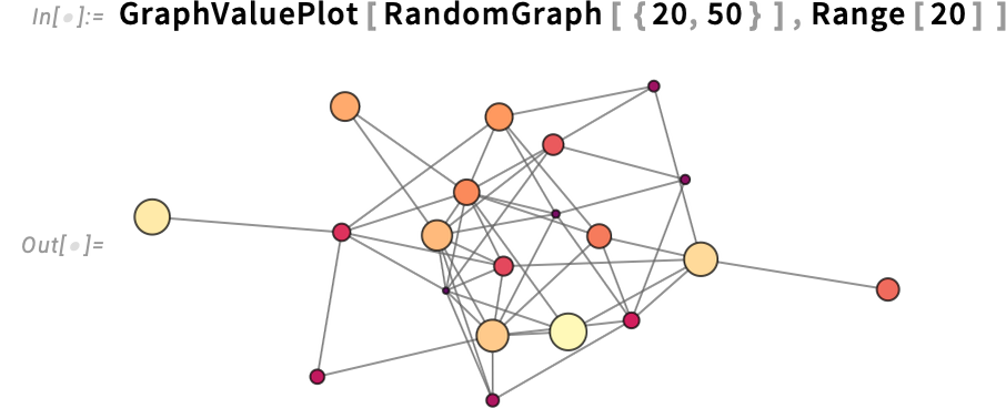
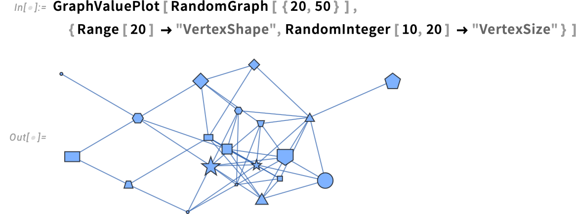
You can represent values in different ways; here we’re saying to just use vertex size
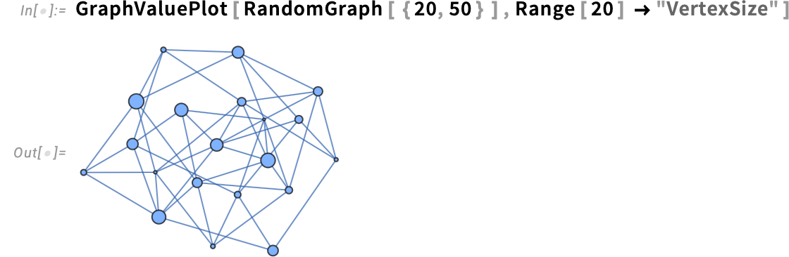
and here we’re using vertex shape as well as vertex size:
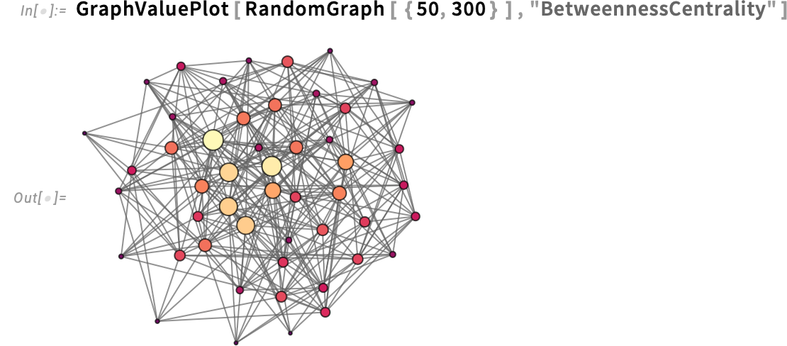
Various standard graph properties are directly supported right within GraphValuePlot. So, for example, this shows a graph with its closeness centrality plotted on it:
GraphValuePlot supports plotting values not only on nodes, but also on edges:
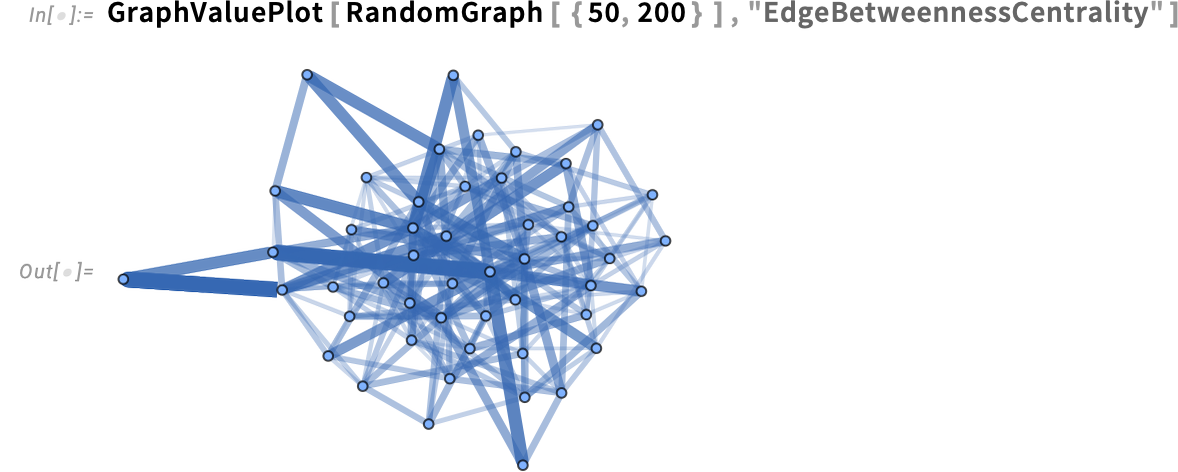
Here’s an example where we’re taking a graph whose edges are annotated with their edge capacity, then plotting these values on the edges:
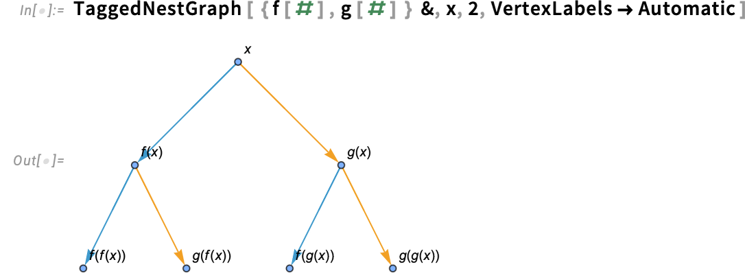
GraphValuePlot takes a graph one already has, and then plots values on it. In Version 15 another new function is TaggedNestGraph—that builds a graph, with tags on its edges, that by default are styled according to those tags. Here’s an example, where the “f” and “g” edges are differently tagged, and differently styled:
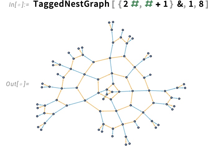
And here’s a slightly larger example:
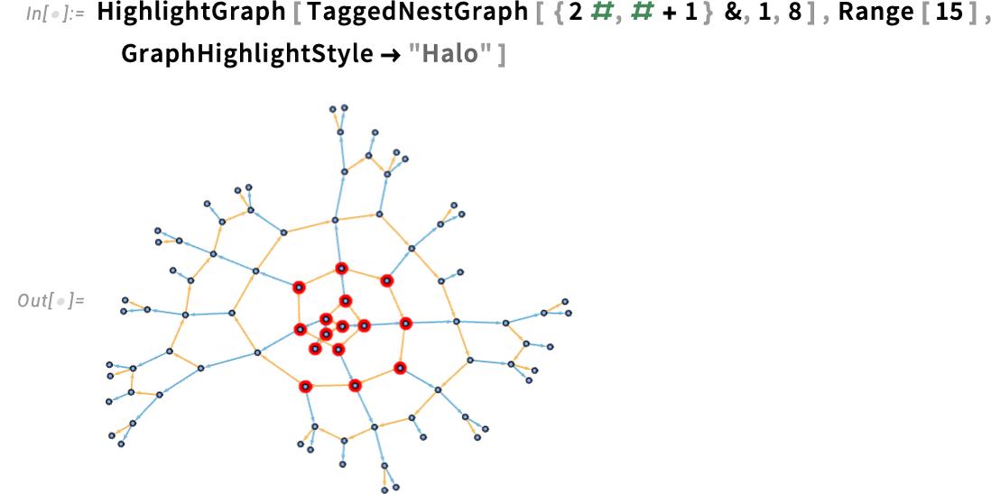
Another thing new in Version 15 is a collection of new highlighting styles for graphs. Here we’re using haloing to highlight some nodes:
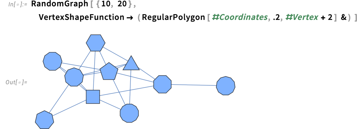
GraphValuePlot is a high-level function for plotting on graphs. But anything it does can also be done at a lower level by explicitly specifying the rendering of vertices and edges in the graph. And at the very lowest level, one has options like VertexShapeFunction which let one, for example, apply a function to completely control the “shape” of every vertex. Of course that can get quite fiddly, not least in having to give vertex coordinates, vertex size and vertex name as three arguments in order. Well, in Version 15 we’ve made that slightly easier, by allowing these values to be accessed from an association, as in #Coordinates, etc.:
How Do You Put Ticks on a Map of the Earth?
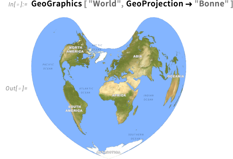
When we make a map of the Earth, we are always in effect projecting the 3D roughly spherical Earth onto a 2D map. There are many ways to do this, as specified for example by the GeoProjection option, an example being:
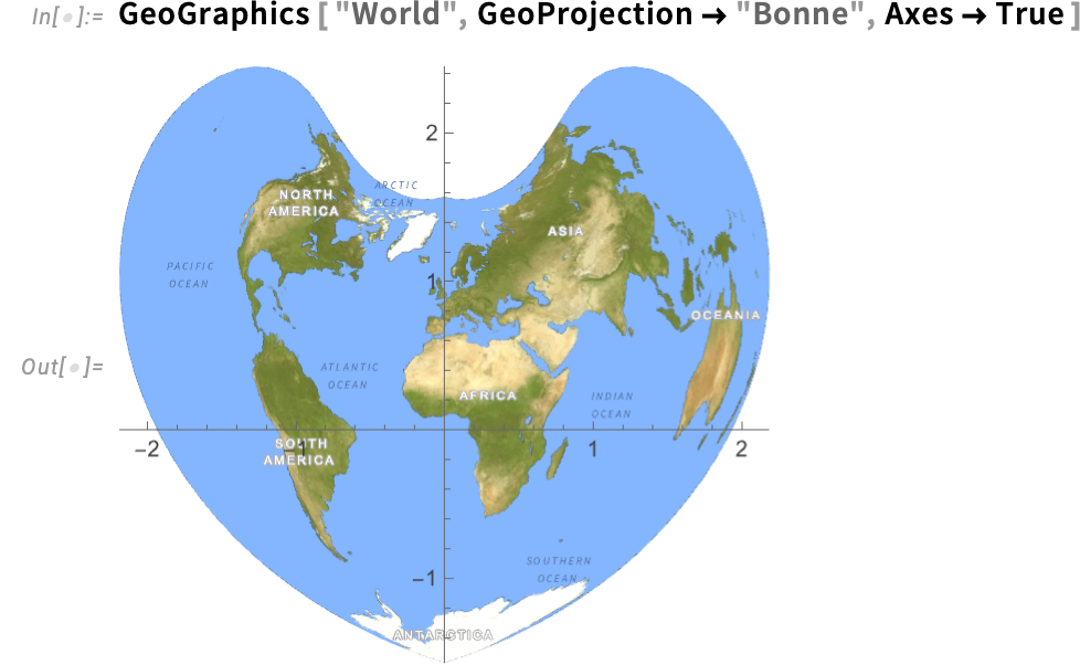
But let’s say we want to read off the coordinates for a point on this map. If we ask to include ordinary axes we get:
The coordinates on these axes are coordinates for the final, projected map. But what if we want to know where points are on the surface of the Earth, say in terms of latitude and longitude? Well, in Version 15 there’s a new option GeoAxes that gives us “geo” or “lat-lon” axes:
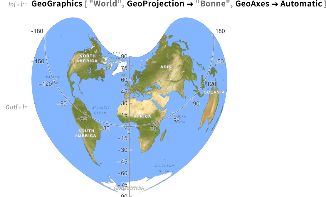
There’s one “geo axis” at the equator; the other, at least by default, is at longitude 0°, i.e. the Greenwich meridian. Along with the geo axes, there are also geo grid lines—which line up with the ticks on geo axes that are present:
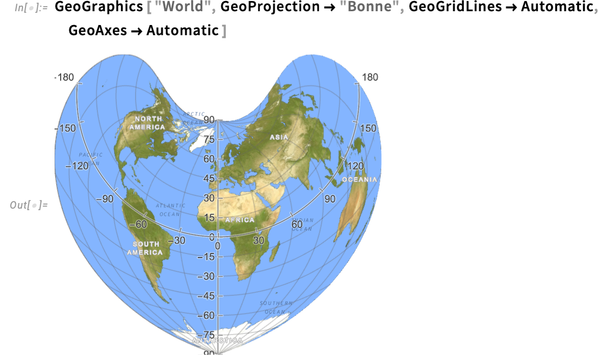
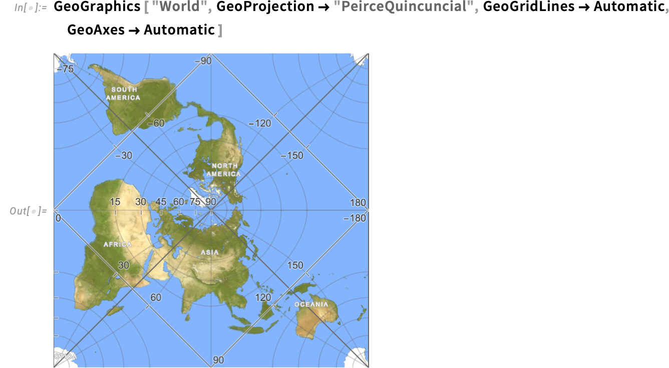
With some geo projections, things can get pretty exotic. Like here the equator is a square:
Oh, and of course, it all works on the Moon (or other planets) too:
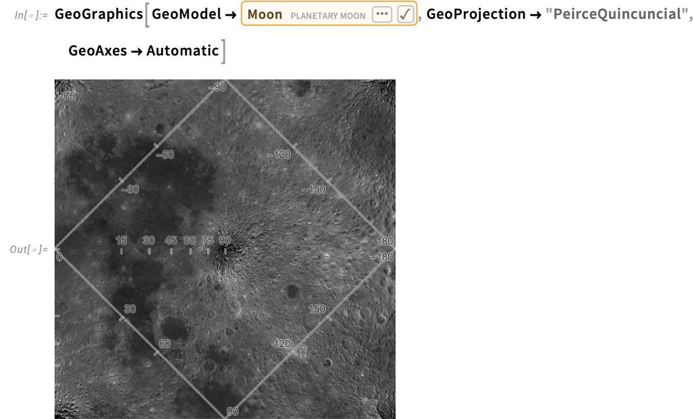
(Internally, this particular projection is an interesting application of the doubly periodic Jacobi elliptic functions JacobiSN, etc.)
There are lots of options for geo axes—like where to make the axes cross (GeoAxesOrigin):
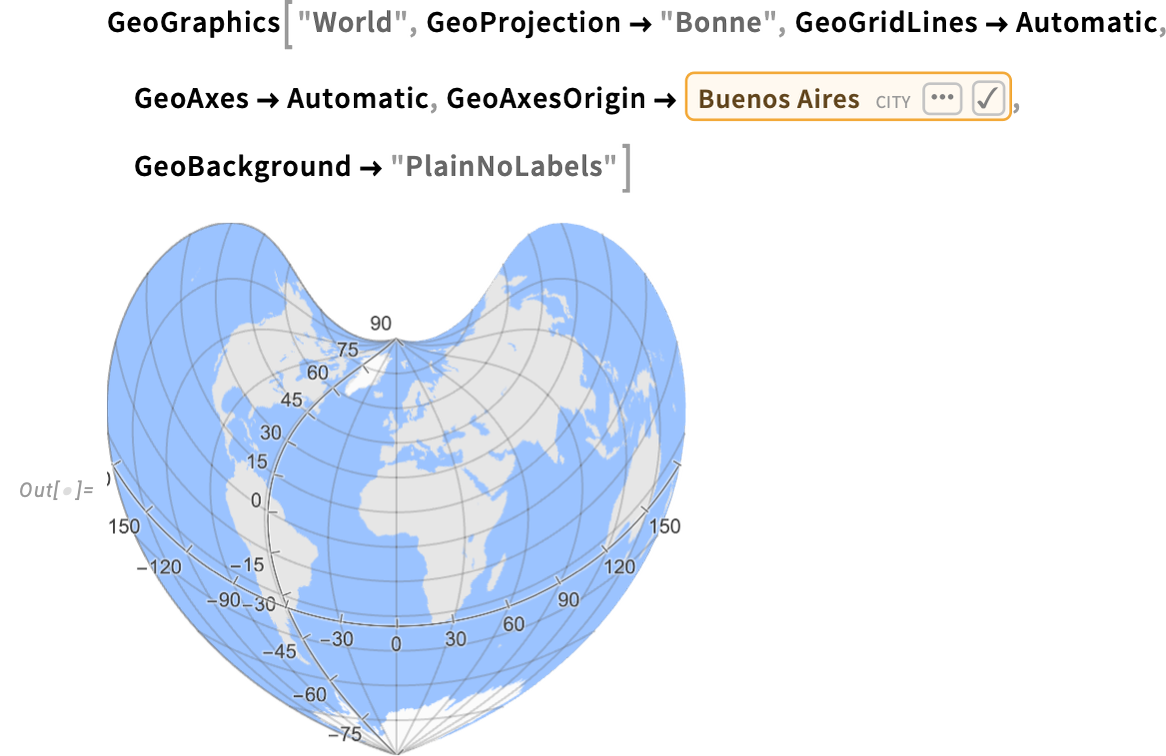
If you want full control over the axes, you specify an AxisObject—and in GeoGraphics, such an AxisObject will be correctly transformed into whatever geo projection you are using.
When Will Your City See a Solar Eclipse?
Astronomical computation has been a driver for the development of exact science for millennia. And historically one of the most challenging problems to be addressed was the prediction of eclipses. And it’s an impressive sign of scientific progress that it’s now possible to predict eclipses to sufficient precision that, for example, in 2017 we were able to have a website that predicted when an eclipse in the US would arrive at any particular point to within one second. What we did was based on the function SolarEclipse that we introduced in 2014—that computes the properties of any specific eclipse within a period of about 30,000 years.
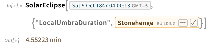
But what about the inverse problem? Given a location on the Earth, what eclipses will be seen there? It’s a challenging problem of both astronomical computation and geo computation. But in Version 15 we’re introducing the function FindSolarEclipse to do this. Here we’re asking when there’ll next be a (non-partial) solar eclipse visible from Stonehenge:
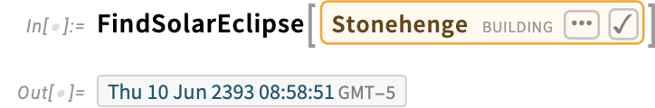
I guess it’ll be a while…. What about in the past?
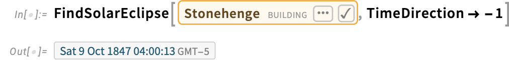
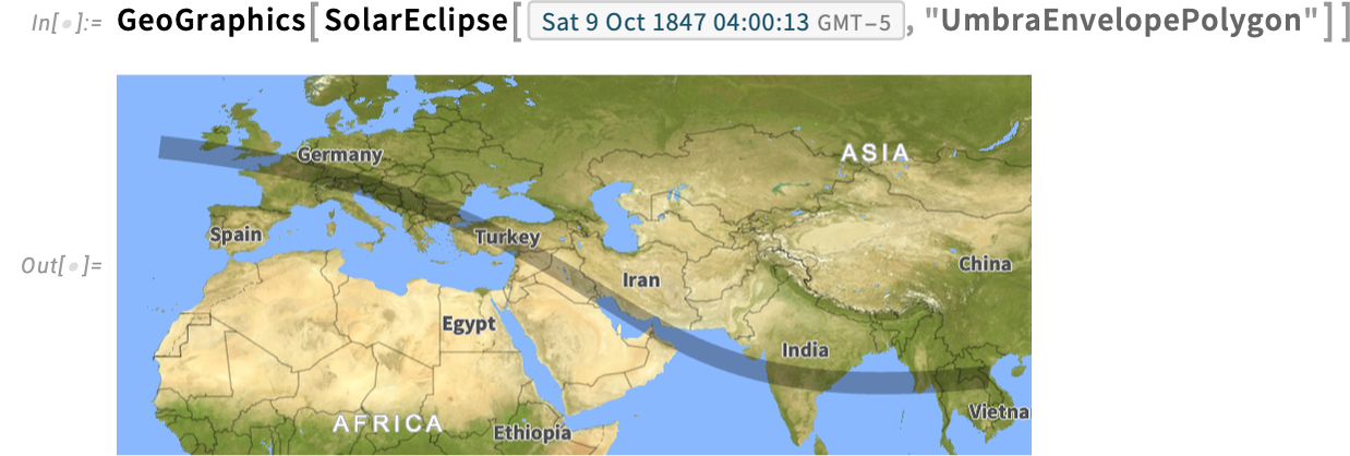
Here’s the path of that eclipse:
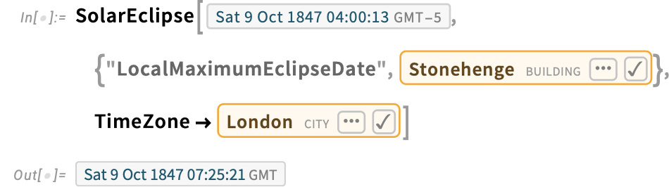
And here’s when the total eclipse reached Stonehenge:
This is how long it lasted:
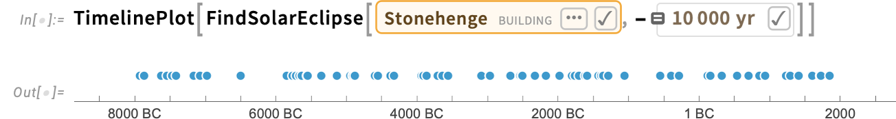
Here’s the timeline of all (non-partial) eclipses visible from Stonehenge over the past 10,000 years:
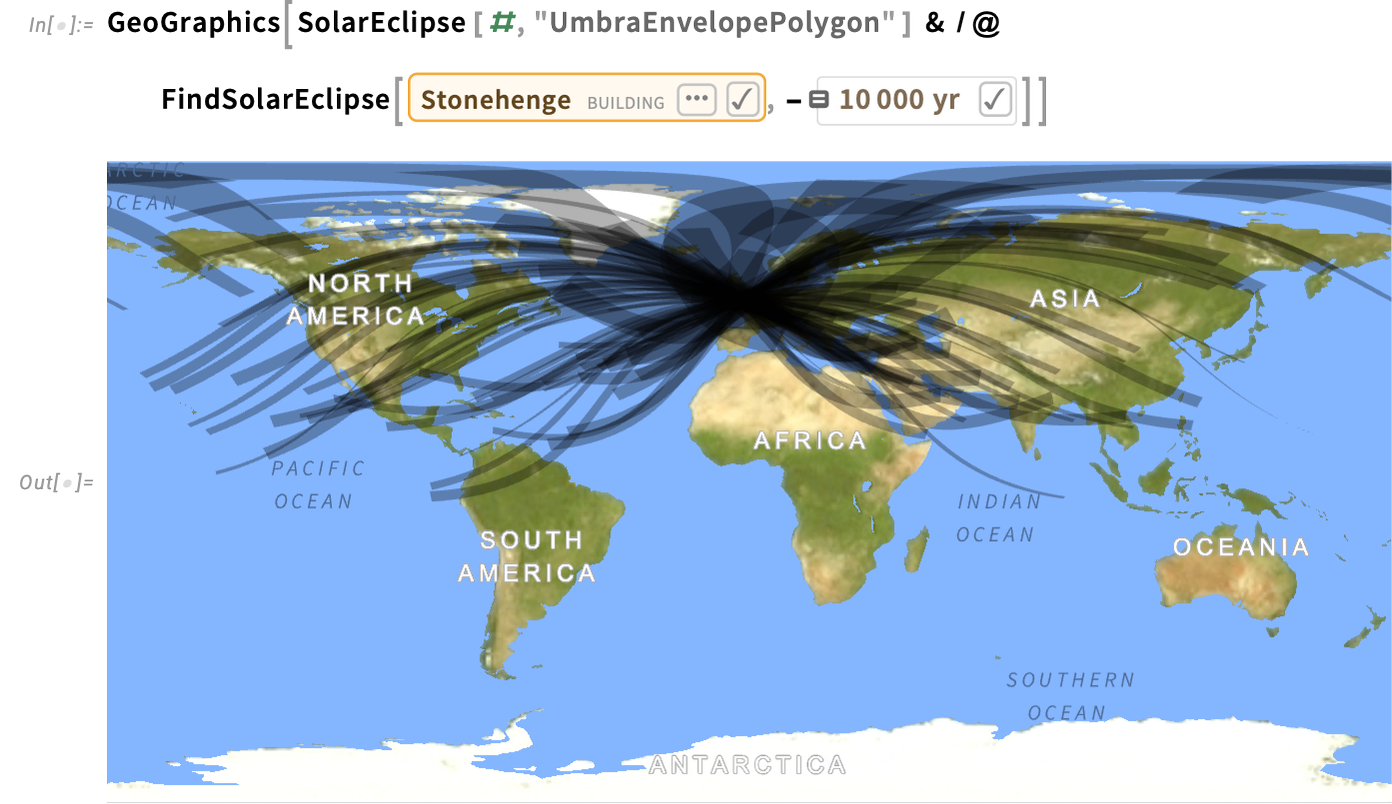
And here are all their paths:
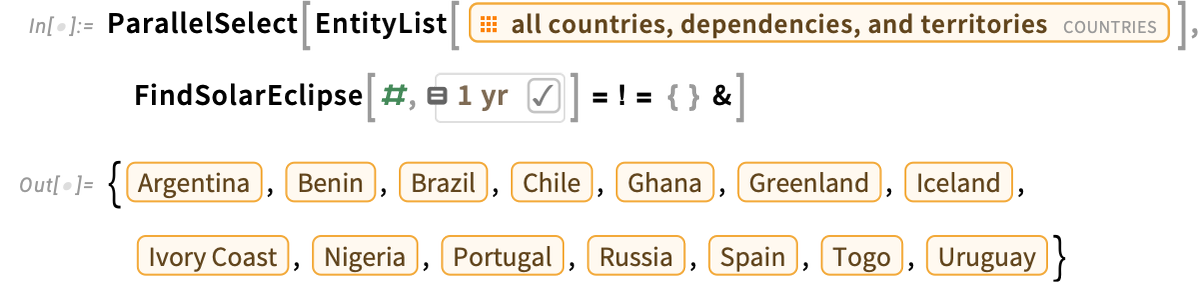
By the way, FindSolarEclipse also works with extended geo regions, like countries:
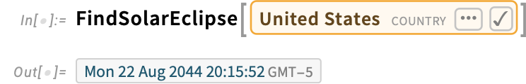
And, yes, for the US it’s going to be a while. But—using quite a collection of capabilities—here’s a list of the countries that will experience a total eclipse in the next year:
Launching into Orbit(s)
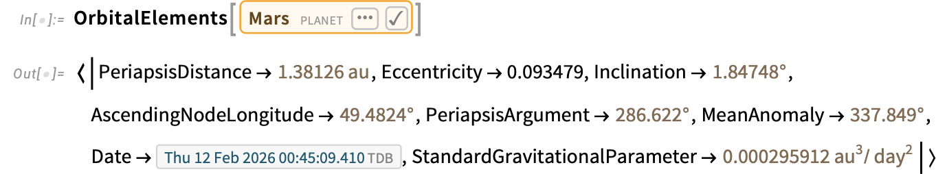
The story of celestial mechanics is, first and foremost, a story of orbits. And in Version 15 we’re beginning the process of supporting computation with orbits. For this version we’re concentrating on (“Keplerian”) orbital elements which in effect give an instantaneous approximation to an orbit. So, for example, for Mars today here are the basic orbital elements we get:
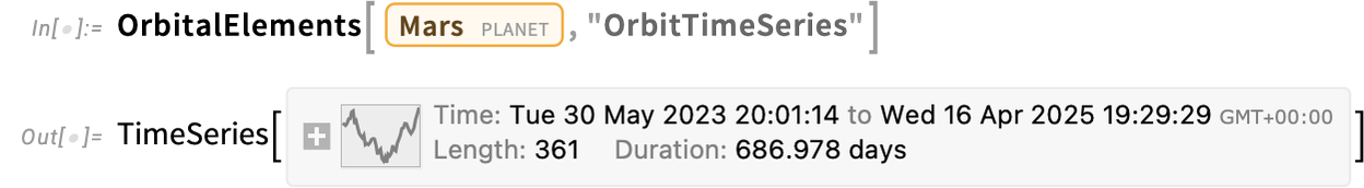
We can think of these orbital elements as giving parameters for the ellipse that best represents the current orbit of Mars. Here’s a time series of that orbit:
And here are the orbital elements predicted for 10,000 years in the future:
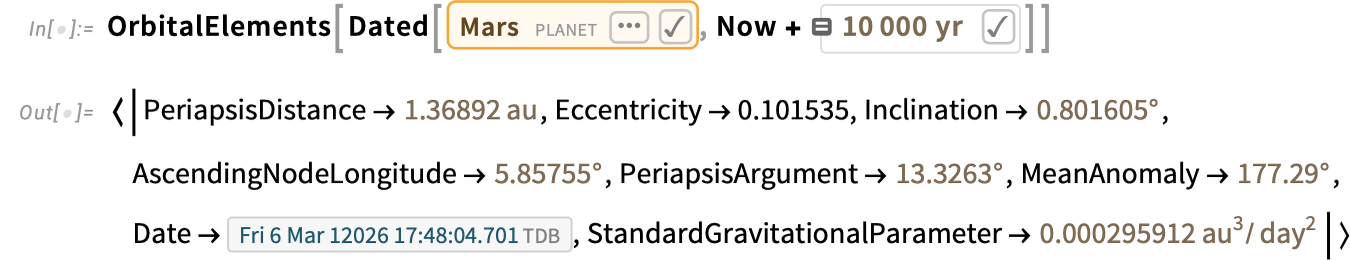
Most of these are very similar to the current orbital elements, indicating that the ellipse approximating the future orbit is very similar to the one for the current orbit. (The “mean anomaly”, though, is basically the angle of Mars within its orbit, so it changes quickly.)
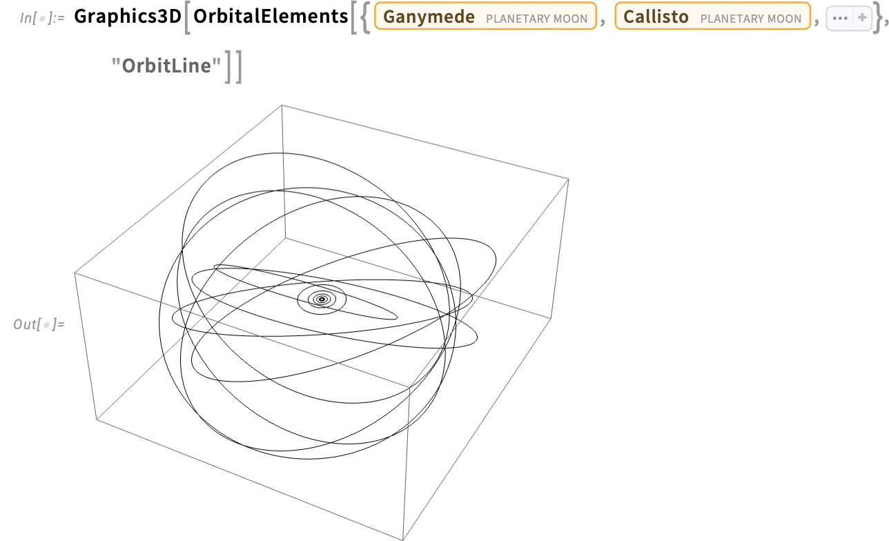
We can compute orbits for planets, moons, minor planets and comets, as well as for spacecraft. Here are the instantaneous orbits computed for inner moons of Jupiter (and, yes, the Galilean moons are some of the ones on the inside with very “little-solar-system-like” orbits):
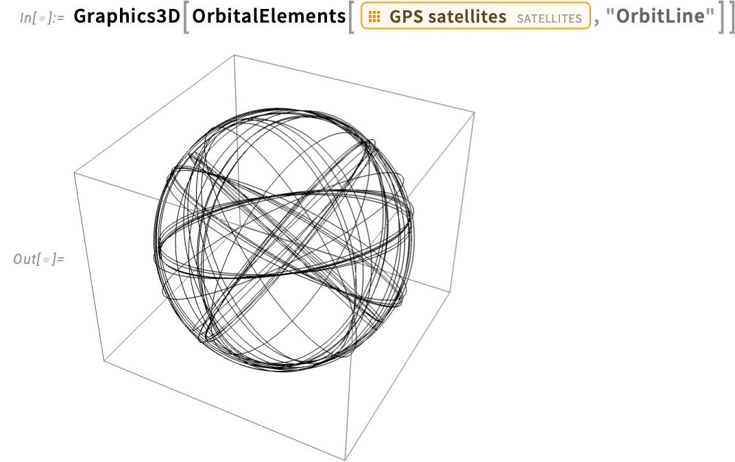
Similarly, here are the current orbits of the GPS satellites, in this case around the Earth:
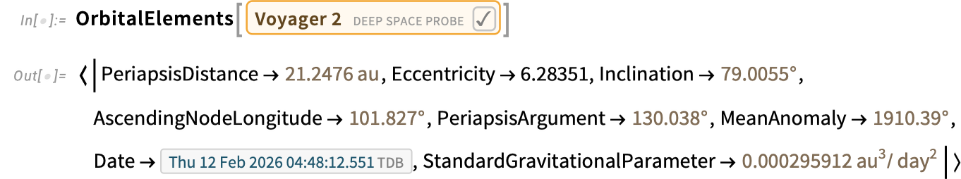
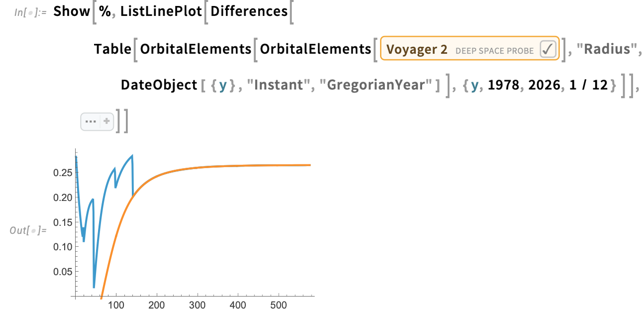
These orbits are all elliptical. But OrbitalElements can also handle hyperbolic orbits—like the path of Voyager 2, which shows a telltale eccentricity larger than 1 (note the relativistically defined TDB time system):
Let’s explore this a bit. Here’s the monthly change in distance from the Sun of Voyager 2 since its launch:
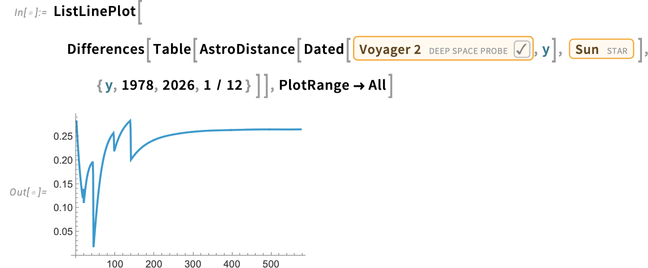
At the beginning there are glitches associated with gravity assists from the planets—followed by a “coasting” phase that corresponds to a hyperbolic orbit. But what is that orbit? Well, it’s the one specified by the current orbital elements for Voyager 2. Taking these and computing the position they imply, we see that indeed the current hyperbolic orbit matches the position—right back to the time of the last gravity assist:
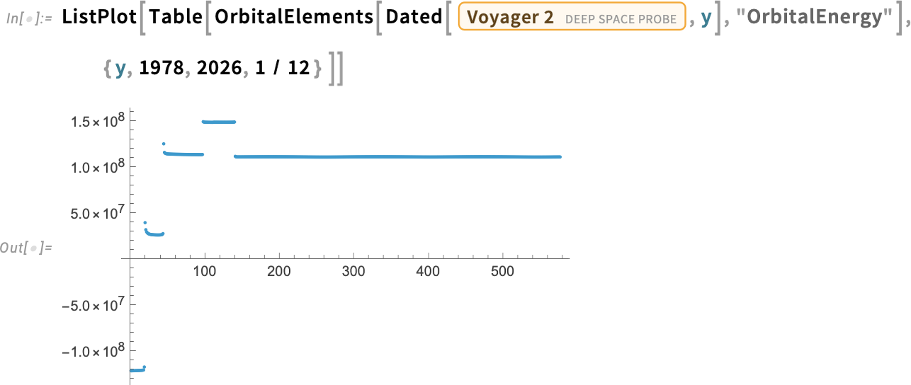
We can compute lots of things from the orbital elements. For example, this shows the total energy in each month—illustrating the fact that the very first gravity assist (from Jupiter) gave Voyager 2 the energy to escape the solar system:
Grassmann, Clifford, Weyl & Friends
What does one mean by “computer algebra”? Traditionally one thinks about operations on things like polynomials where the variables (say x) are ultimately supposed to represent numbers. But what about other kinds of algebras, where, for example, the multiplication operation isn’t commutative?
In Version 14.3 we introduced non-commutative computer algebra for free algebras—with symbolic matrices being a notable example. Now in Version 15.0 we’re introducing non-commutative algebra for algebras with relations, in particular Grassmann, Clifford and Weyl algebras.
So, for example, GrassmannAlgebra represents a Grassmann algebra
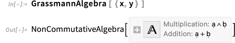
with the (non-commutative) multiplication operation being ⋀ (typed as \[Wedge]). In a Grassmann algebra multiplication is defined to anticommute, and NonCommutativeExpand will attempt to put variables in the order they are specified for the algebra (here x followed by y) so that for example:
CliffordAlgebra represents a Clifford algebra
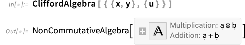
in which, in this case, x and y are defined to “square” to 1, while u is defined to “square” to –1:
(The non-commutative multiplication ![]() can be typed as **.)
can be typed as **.)
Then there’s WeylAlgebra, which is convenient in representing compositions of differential operators, here in effect “expanded” by using the chain rule:

You can also define your own non-commutative algebra with relations:
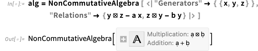
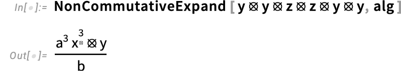
(There’s a lot to say about all this; in fact, there’s now a whole Wolfram monograph entitled “Non-Commutative Algebras” about it.)
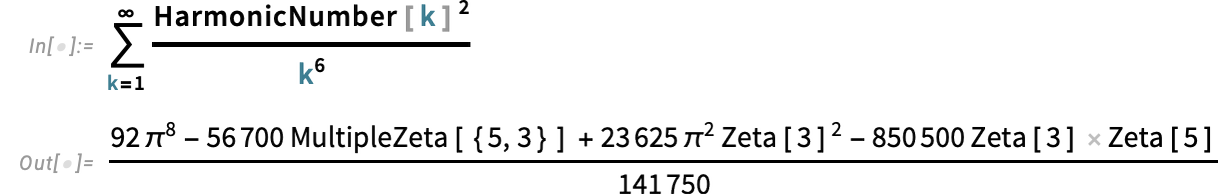
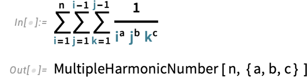
Zetas, Polylogs and Harmonic Numbers Go Multivariate
“Is there a closed form for that?” Well, it depends what one means by “closed form”. But operationally it tends to mean “Can the result be represented in terms of functions we’ve defined?” And the answer to that, of course, depends on what functions one’s defined. And in every new version of the Wolfram Language we try to add new “special functions”, that can help us provide closed-form solutions to a larger class of problems.
Well, in Version 15 we’re adding a collection of particularly powerful new special functions that let us substantially extend the range of closed-form results we can get, particularly for applications in quantum field theory and analytic number theory. The basic story of these new special functions is that they’re multivariate generalizations of the Riemann zeta function, polylogarithms and harmonic numbers. But they turn out to appear rather widely in series solutions of systems of linear differential equations, in integrals of multivariate rational functions and in multivariate sums.
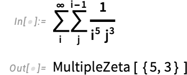
We’ve had ordinary, univariate zeta functions since Version 1:
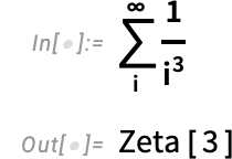
When they’re simple enough, multivariate analogs of sums like this can still be done in terms of univariate zetas:
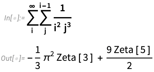
But in general they need our new MultipleZeta function:
And, yes, things can get complicated pretty quickly
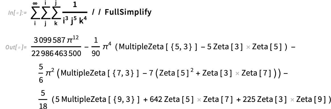
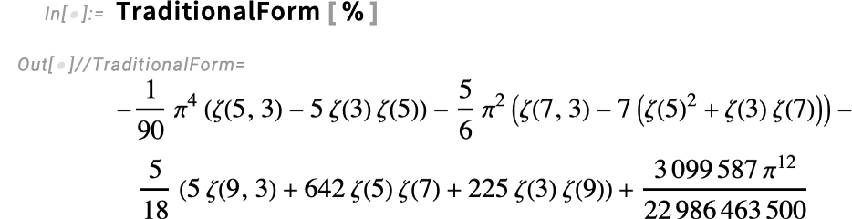
though in TraditionalForm the result is at least fairly compact:
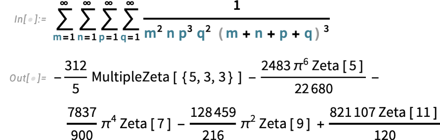
Here’s an infinite sum that involves a trivariate zeta:
And here’s a univariate sum that still involves a multiple zeta:
One can think of polylogarithms as being like zetas but with a “power series numerator” added:
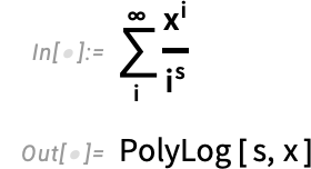
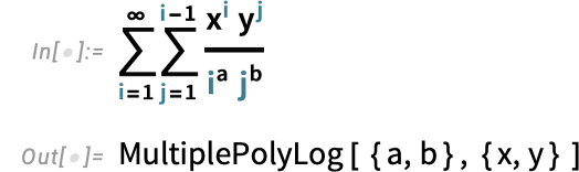
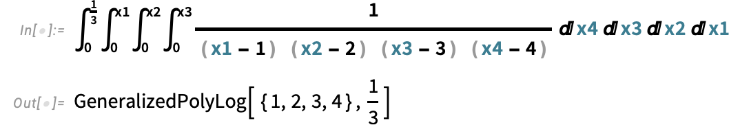
There are then several ways to generalize polylogarithms to the multivariate case. The most straightforward is what we’re calling MultiplePolyLog:
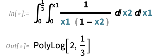
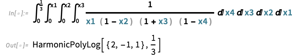
But to cover other cases that often show up we’re also adding what we’re calling GeneralizedPolyLog and HarmonicPolyLog. Ordinary PolyLog can be obtained from a univariate integral such as
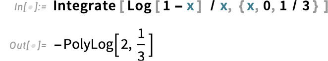
or a bivariate integral such as:
And when we extend this to more variables we start getting our new kinds of polylogarithms:
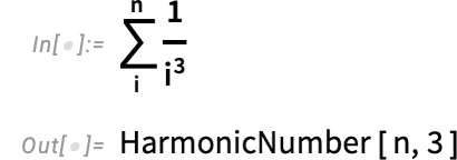
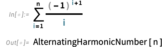
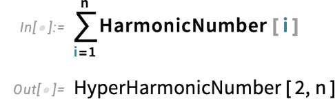
The third type of function that’s “going multivariate” in Version 15 is HarmonicNumber:
And we’re also adding some new univariate kinds of harmonic numbers, such as:
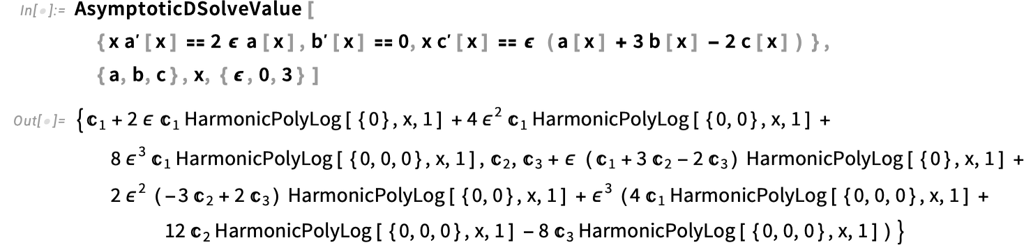
But in the end what’s most important about these new special functions is how wide range the range of computations in which they show up is. Like here’s the result for an asymptotic expansion of the solution of a differential equation (that happens to come from a Feynman diagram) that’s full of harmonic polylogarithms:
Partial Fractions Get Streamlined
We’ve had the function Apart ever since Version 1.0. But now in Version 15 we’re “taking apart Apart”, making it more algorithmically precise and sophisticated—and giving access to more parts.
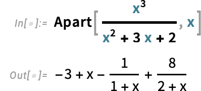
The core operation behind Apart is computing partial fractions—and now there’s a specific function for that:
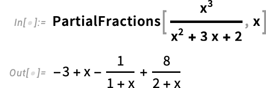
In this particular case, the result is the same as from Apart:
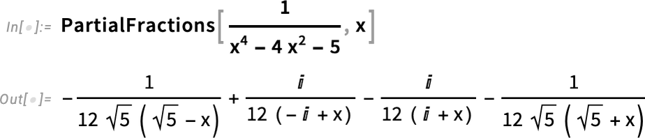
But in this case
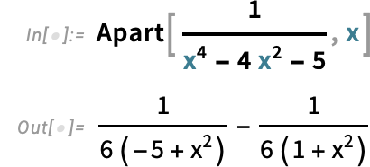
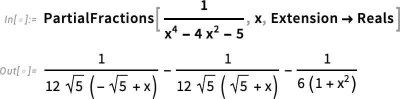
Apart stops when it can no longer factor denominators over the rationals, but PartialFractions by default keeps going, here using complex roots to do complete factorization:
If you don’t want complex roots, you can tell PartialFractions to only use Reals:
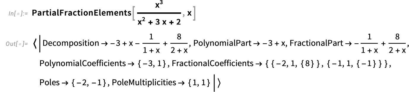
Partial fractions get used in many symbolic algorithms (starting with the original method for integrating rational functions back in 1703)—and in different cases different parts of the results are what’s needed. So in Version 15 we’re introducing PartialFractionElements to give direct access to different parts:
Lots of New Matrix Decompositions
At some level, matrices are just arrays of values, or, in the Wolfram Language, lists of lists. But depending on what a matrix is going to be used for, there are often other representations that do much better at capturing its “algorithmic essence”. And that’s where matrix decompositions come in. We’ve had functions for a number of the most common matrix decompositions since the early 1990s. But in Version 15 they’re being updated and streamlined, and some powerful new ones are being added.
A typical example of a matrix decomposition (that happens to be new in Version 15) is LDLDecomposition—where we take a matrix and decompose it into “L” and “D” pieces:
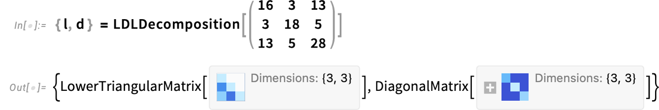
We can reconstruct the original matrix from these pieces:
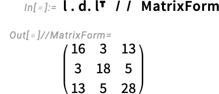
But the point is that if we’re using the matrix to represent linear equations, then the “L” and “D” pieces are what we need to immediately be able to efficiently solve them. We could in principle always get a solution by applying LinearSolve directly to the original matrix:
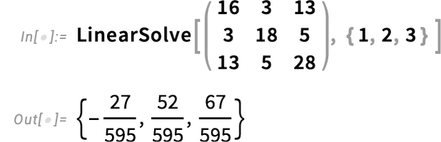
But it’s much more efficient to use the “L” and “D” pieces
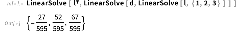
because with triangular and diagonal matrices LinearSolve has to do vastly less work.
A function like LDLDecomposition by default makes use of new structured matrix objects like LowerTriangularMatrix—that optimize the storage and computation of matrices with particular forms. (The option TargetStructure lets you control what kind of matrix structure will be used.)
One matrix decomposition that we’ve had since Version 3 is LUDecomposition. But now in Version 15 it’s able to use structured matrices—which makes it both more efficient and more convenient:
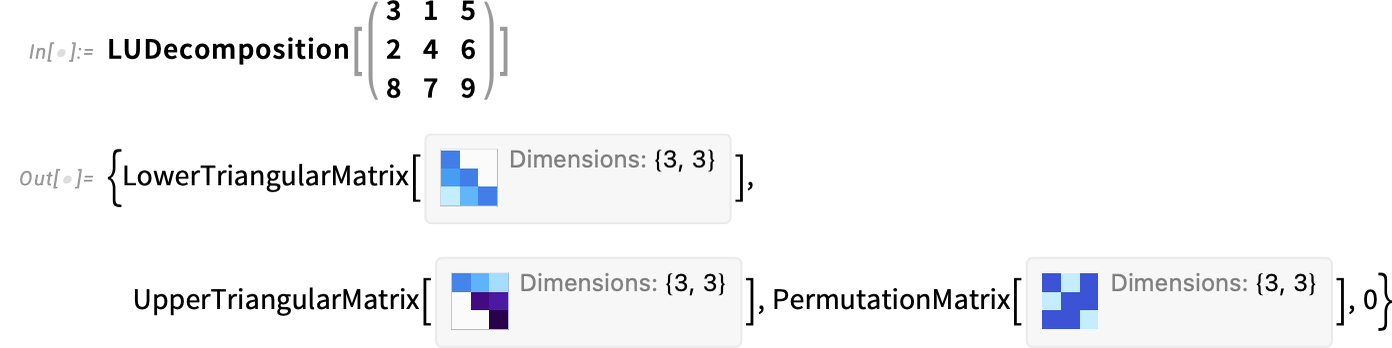
Another new matrix decomposition is RankDecomposition—which factors a rank-k m×n matrix into m×k and k×n matrices
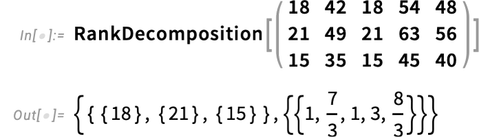
from which the original matrix can be reconstructed with Dot:
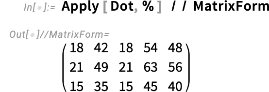
Other new matrix decompositions include BunchKaufmanDecomposition and PolarDecomposition. In addition, there are new functions like JordanReduce and FrobeniusReduce that give the “core” of JordanDecomposition and FrobeniusDecomposition.
The Corners of DSolve Get a Little Help from AI Methods
“Won’t AI just solve it all?” The surprise success of ChatGPT back in 2022 made many people wonder just how far AI systems (and specifically neural nets) might be able to get in every area—including math. Elsewhere, I’ve talked about the science of this. But suffice it to say that there are places where there’s no way to avoid deep computation, which is something neural nets aren’t set up to do (well, unless they call tools like Wolfram Language). But there are still places—potentially even in math—where it’s reasonable to think that kind of broad “heuristic” computation that neural-net AI does might be relevant.
There are of course plenty of functions in the Wolfram Language that have been using neural nets for a long time (think ImageIdentify, SpeechRecognize or FeatureSpacePlot). But not specifically math functions. Still, we’ve been exploring the possibilities for a while now, and in Version 15, for the first time, we are starting to use neural-net methods inside a symbolic math function, specifically DSolve.
One can think of neural nets as fundamentally doing approximate computation. So how can one use that for a function like DSolve that produces exact, symbolic results? The basic idea is to use a neural net to “guess” a possible solution, then to use precise symbolic computation to test it, only returning it as a result if it checks out.
It’s worth mentioning that we actually have many very powerful algorithms for symbolic computation in Wolfram Language (often ones we’ve invented) that use approximation (often, numerical approximation) inside—and then use precise symbolic methods to filter or validate the result. But DSolve in Version 15 is the first time we’re specifically using neural nets inside a symbolic mathematical computation function.
What is the fundamental problem DSolve is trying to solve? It’s given a differential equation, then asked to find a function—preferably one that’s structurally as simple as possible—that solves the equation. So how can one train a neural net to do that? The basic idea is to generate lots of functions, then find differential equations that they satisfy, then provide the differential equations and the functions we know solve them as training data for the neural net.
How does one encode a mathematical expression for a neural net? We’re essentially treating the math like natural language, and turning it into a string of tokens. And the neural nets we’re using are transformers, just like in LLMs.
So what’s the result? Here’s an example of a differential equation that Version 14.3 couldn’t solve, but—thanks to our new neural net method—Version 15.0 can:
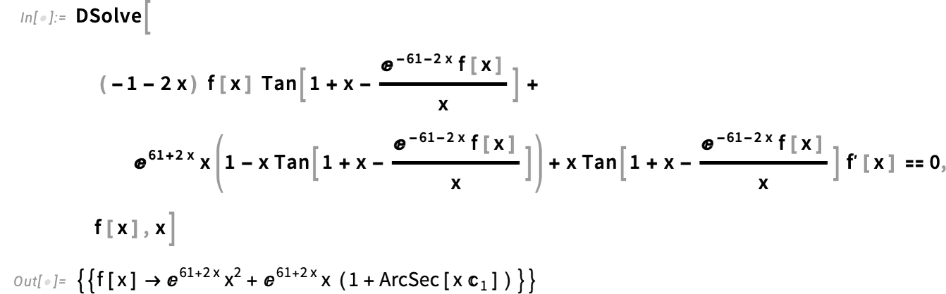
And, yes, this looks like a bit of a put-up job: a very complicated equation that “just happens” to have a solution. And, yes, that’s a valid criticism. And it raises the question of what the distribution of differential equations one might actually want to solve will be. From Wolfram|Alpha we actually in principle have quite a lot of information on that. And we’ve been accumulating benchmarks from things like books of tables for a long time. So how do neural nets do on those? Not terribly well. For example, out of the 638 (first-order) differential equations in the classic 1959 Kamke handbook, our neural net method can solve just 6. Our “traditional” algorithmic methods, on the other hand, get 100% of the solutions.
But what if we just “synthetically” generate equations to solve? We can do the same thing we did in generating training data, and probabilistically generate expression trees (essentially using a Markov process whose transitions are applications of named functions, like Sin and Log)—then find equations these expressions satisfy. And if we generate a million equations this way, we find that, yes, the neural net can find correct solutions to about 80% of them. But—and here’s the kicker—our traditional algorithmic methods can also find almost all these solutions. And in the end, only 0.003% of our test equations can successfully be solved by the neural net, but not by our traditional methods. So does that mean the neural net is basically useless? Well, it’s always nice to be able to solve a few more equations (even 0.003% more). But there are two things that make the neural net more useful. First, when it works, it often gets an answer significantly faster than our traditional algorithmic methods can. And, second, there are a significant number of cases where the answer it gives is considerably simpler than what traditional algorithmic methods could find.
Here’s an example of what DSolve did in Version 14.3 with a particular differential equation:
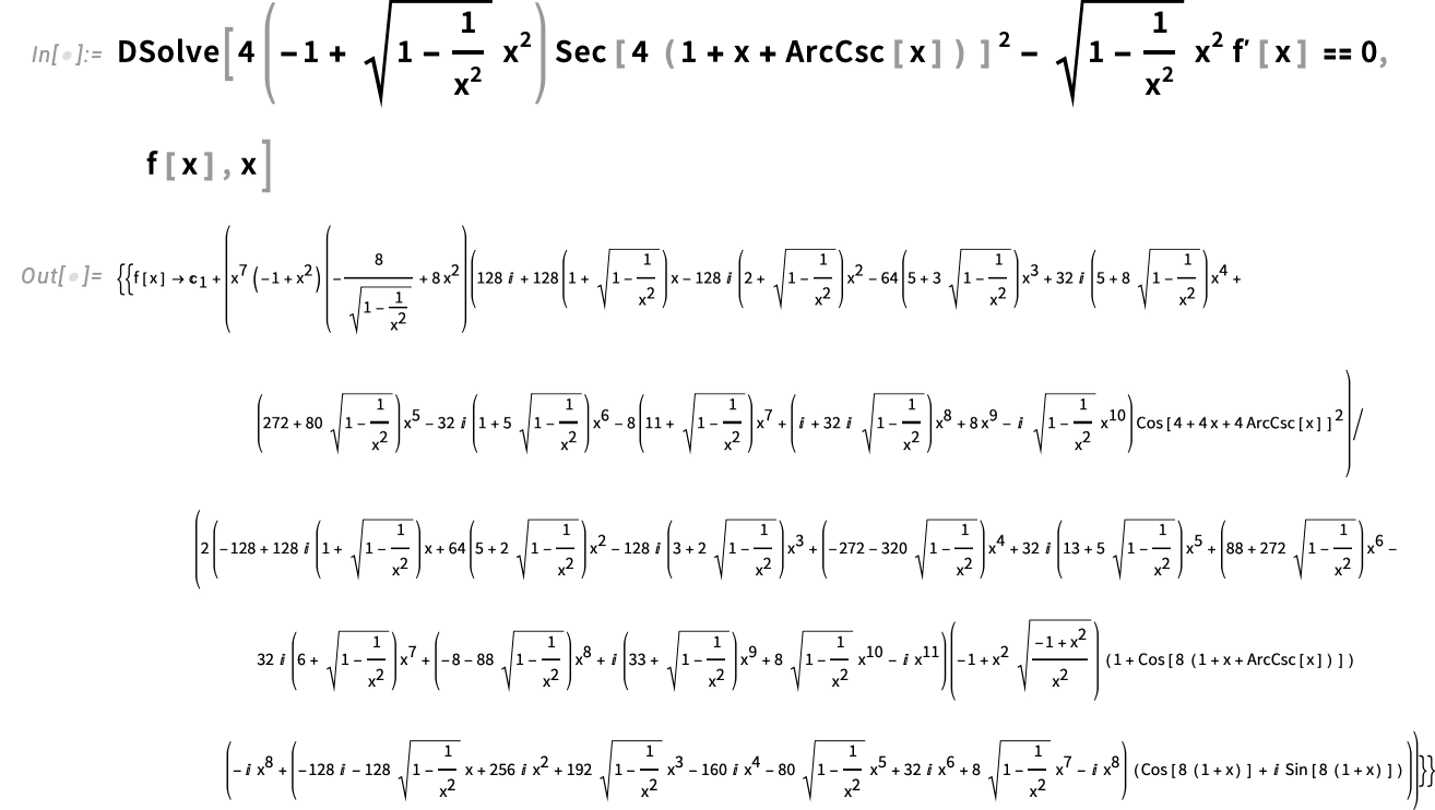
If we apply FullSimplify, then after several minutes we get:
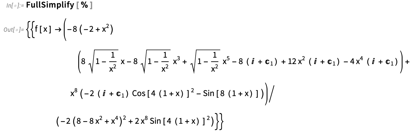
But now in Version 15.0, here’s the result we get, courtesy of our new neural net method:
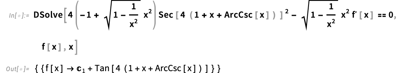
It’s a lovely, elegant result. Of course, it’s fairly close to things that appeared in the training data we provided. But the neural net has done what neural nets do best: it’s in effect successfully made a model for what solutions to the kind of differential equations it’s seen are like, and it’s able to use that model to do a certain amount of generalization.
For sure it’s a nice demo. And it could well be that a differential equation that comes up in some practical setting will now be able to be solved symbolically when it couldn’t be before. It’s hard to tell. But for us it’s already interesting that we’ve been able to put a neural net method into a core mathematical function in the Wolfram Language. And the pipeline that we’ve built for doing that we’ll be applying wherever it makes sense in the future.
(By the way, you might wonder whether the new solution and old are in fact the same. Both contain an arbitrary constant ![]() . But if we take their difference, FullSimplify can successfully show that it’s precisely
. But if we take their difference, FullSimplify can successfully show that it’s precisely ![]() . In other words, the difference is a constant which—for a linear equation like this—can be absorbed into
. In other words, the difference is a constant which—for a linear equation like this—can be absorbed into ![]() . So, yes, the solutions are the same, even though they’re algebraically stated in different forms.)
. So, yes, the solutions are the same, even though they’re algebraically stated in different forms.)
PDEs Go Curvilinear
Back when we introduced basic vector analysis functions like Div and Grad in Version 9 we also introduced the idea of coordinate charts—so that, for example, you can compute the Laplacian in polar coordinates:
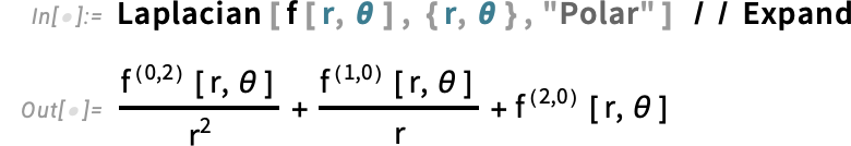
In Version 15 we’re now extending support for coordinate charts throughout our PDE modeling system. So, for example, here’s the Laplacian in polar coordinates computed from a LaplacianPDETerm:
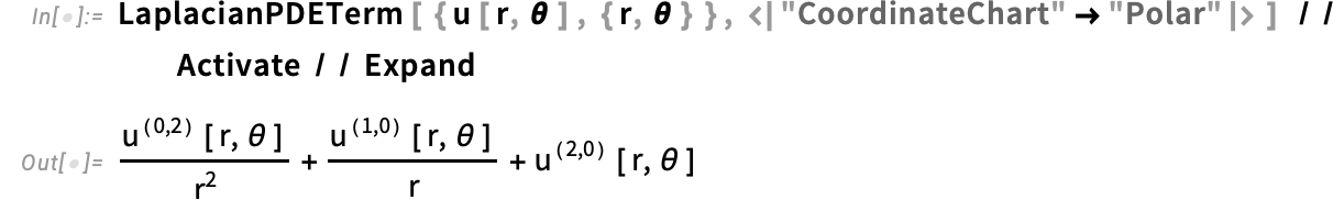
We can put this PDE term into a whole PDE, and solve it, all in polar coordinates:
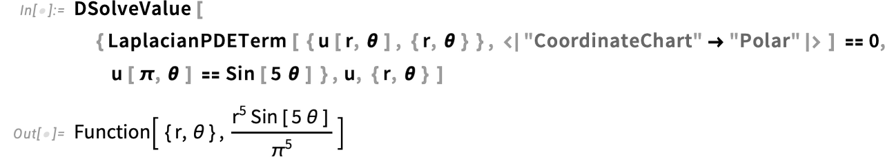
This is all comparatively straightforward for something like a Laplacian with a scalar field, but things quickly get more complicated. Here’s a fluid flow PDE component in polar coordinates:
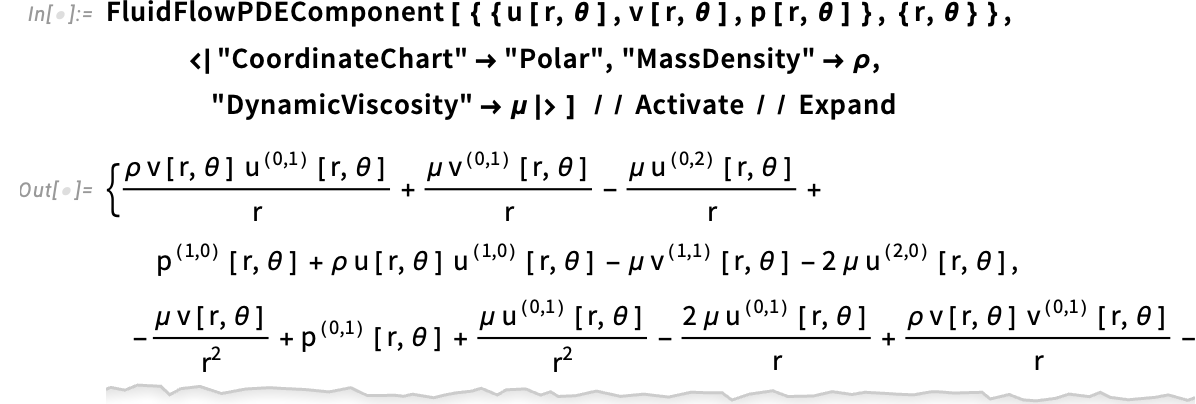
And indeed this works for any curvilinear coordinate system supported by CoordinateChartData. Here it is for spherical coordinates:
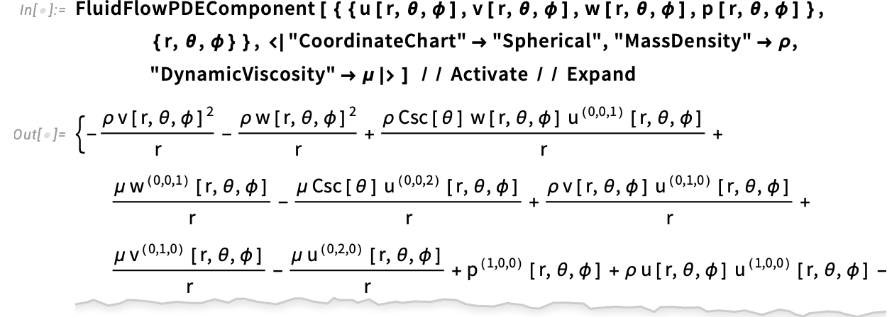
And here for prolate spheroidal coordinates:
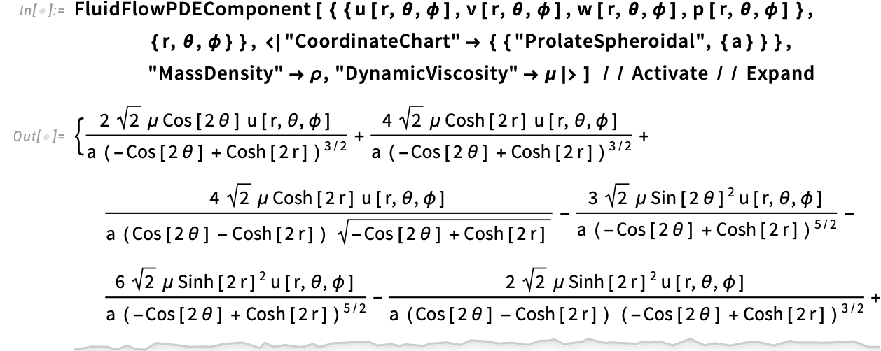
In Version 15 one can now also use curvilinear coordinates for numerical PDEs. Here’s an eigenvalue problem set up and solved in polar coordinates (note that the boundary conditions are also now in polar coordinates):
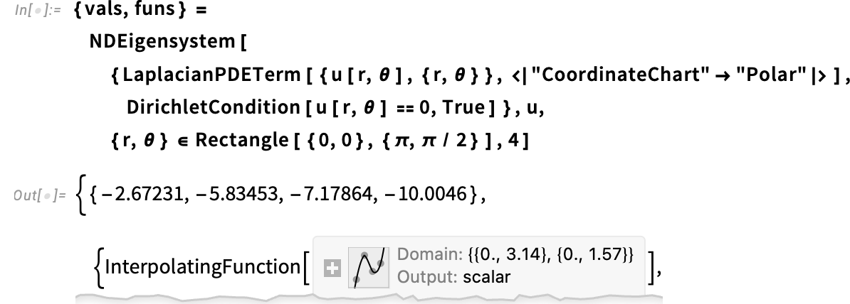
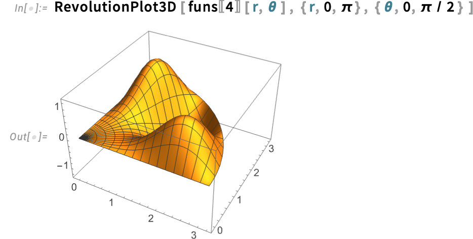
Derived Quantities in PDE Solutions
Let’s say you’re solving a problem in solid mechanics, using PDEs set up with things like SolidMechanicsPDEComponent. The quantity you directly compute is the displacement field—which gives the displacement in each direction at each point in the solid:
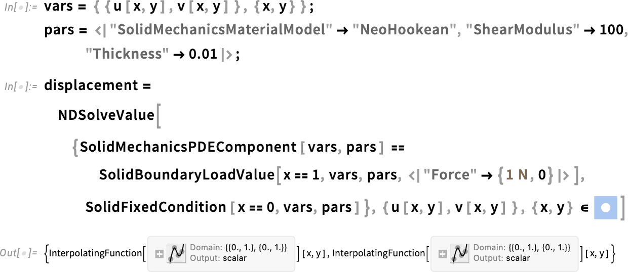
But often what you actually want is some quantity derived from this. So, for example, this computes the strain field corresponding to this displacement field:
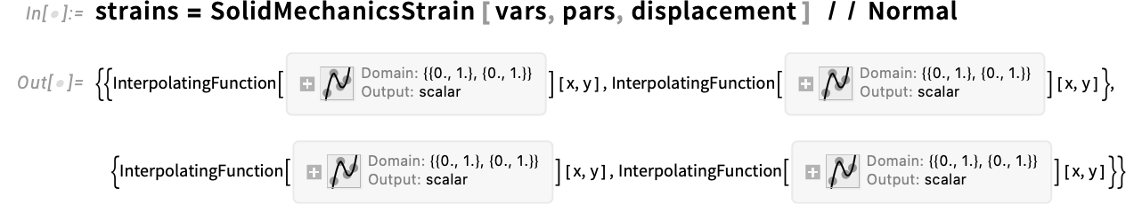
But this corresponds to a complicated rank-2 strain tensor at every point. And it’s common to want to reduce the solution further, say deriving from it some pure scalar quantity at every point. In Version 14.1 we introduced VonMisesStress to do something like this for the stress field. In Version 15 we’re now introducing EquivalentStrain to do it for the strain field:
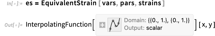
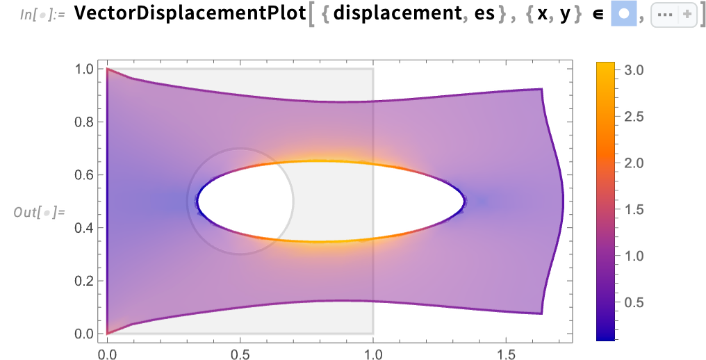
By the way, this is what EquivalentStrain actually does—seen here in symbolic form:
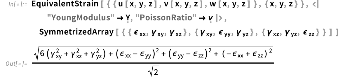
In addition to EquivalentStrain for solid mechanics, Version 15 introduces FluidViscousStress and FluidViscosity for fluid mechanics, and MagneticFluxDensity (“B field”) and MagneticFieldIntensity (“H field”) for studying magnetic fields.
How Do You Approximate a Systems Engineering Model?
There are power series. There are interpolating functions. There are basic neural nets. All can be thought of as providing faster-to-use-than-the-thing-itself approximations to things. But let’s say you have a systems engineering model, represented by SystemModel, and perhaps coming from Wolfram System Modeler. How can you get a faster-to-use-than-the-thing-itself approximation to that?
Version 15 introduces the function SystemModelSurrogateTrain to use modern machine-learning methods to create such approximations. The basic idea is to select some part of the behavior space of a system model, and then to do a series of simulations and fit the “synthetic data” they produce to get what is ultimately an efficient continuous-time neural-net approximation to the original model.
As a simple example, consider a model of an electric motor:
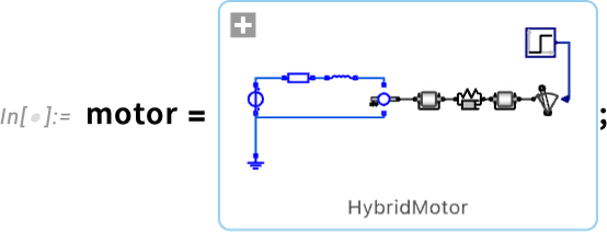
Here’s a plot of the behavior of a particular variable computed from this model with a specific value for a parameter:
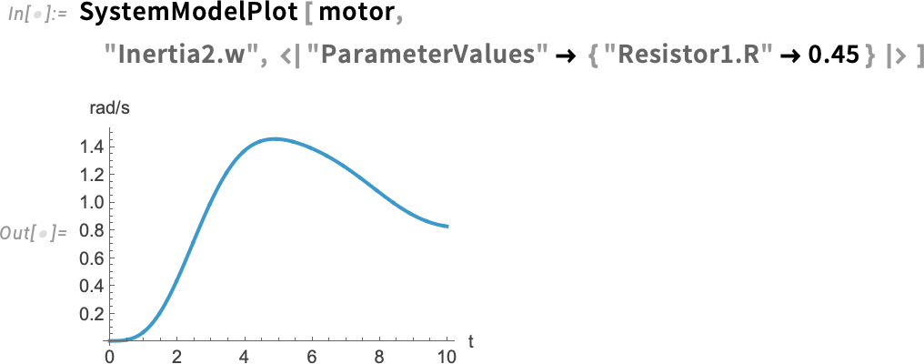
SystemModelSurrogateTrain lets you make a “surrogate” approximation of the underlying model, that efficiently captures the behavior of particular variables in the model for a certain specified range of parameters:
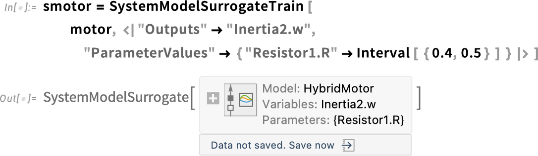
If we do the same computation as above we get essentially the same result—but much faster:
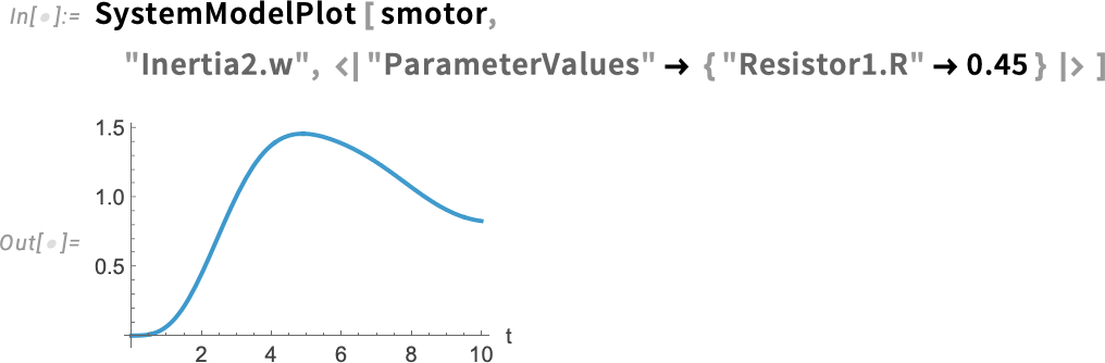
Instead of solving differential equations to get the result, the surrogate model just evaluates a neural net, which we can extract from the SystemModelSurrogate object:
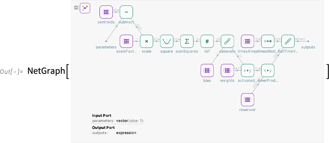
Surrogate models become more and more important for more and more complex engineering systems—and are crucial in making practical many kinds of large-scale system optimization, as well as in making possible digital twins that can be simulated in real time.
Reinforcement Learning for Control Systems
Reinforcement learning has been much discussed in the context of AI in recent years. But the concept actually originated in the 1950s—under the name “optimal control”—in the study and design of control systems. In traditional control theory—that we’ve supported in Wolfram Language for many years—the basic idea is to have a mathematical-style model of a system, and then to operate on the structure of this model to derive a controller that (as far as possible) makes the system achieve specified objectives.
In reinforcement learning, on the other hand, one doesn’t rely on having a mathematical-style model of a system. Instead, one just assumes that one will find out about the system by repeatedly “poking it” and seeing how it responds—and then iteratively come up with a controller that achieves the objectives one wants. There are different strategies for doing this; in Version 15 we’re introducing a powerful one known as Q learning.
The basic idea of Q learning is to constantly try to learn the “Q function” that specifies the “quality of response” associated with a given (control) action when the system is in a given state—and then to take this learned Q function and derive a controller from it. In Version 15 we’re introducing the function LQRegulatorTrain to do linear-quadratic-regulator-based Q learning (and, yes, the “Q” in LQRegulatorTrain isn’t the same as the “Q” in Q learning; it stands for “quadratic” not “quality”).
LQRegulatorTrain takes a representation of the system (usually in reinforcement learning called the “environment”), and tries to minimize a quadratic form that’s accumulated over the course of the reinforcement learning process, and that contains terms associated with the distance to achieving a particular state for the system, and the amount of control used.
Typically the way one represents the system is to give a function which takes the current state (say x) of the system (at a given step, say k) along with a certain input (say u), and then returns a new state of the system. As an extremely simple example, we can use a system specified by the function:
We can now train an LQ regulator to be a controller for this system:
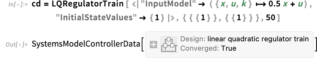
The result is a symbolic representation of a controller. We can take this and for example see how the controller “drives the state response to zero”:
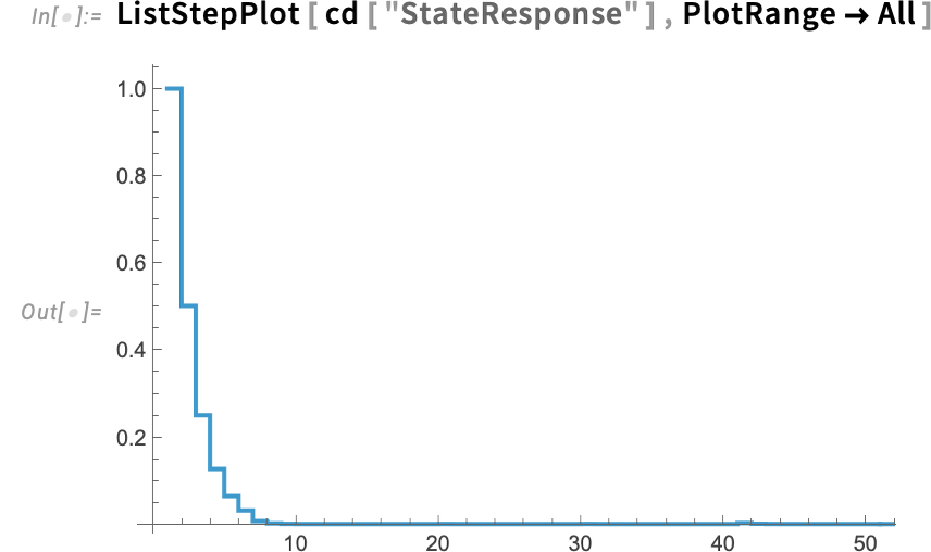
If we want to, we can actually get the Q function itself for this case (which, because this is from an LQ regulator, is a quadratic form):
As a slightly more realistic example, consider a DC electric motor that one’s trying to control to turn a pointer to a particular angle. One can represent this symbolically as a SystemModel:
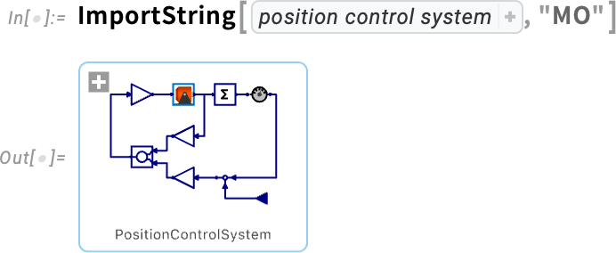
We could have an actual physical version of this, then use our device framework (with functions like DeviceRead and DeviceWrite) to connect to sensors and actuators (or use our Microcontroller Kit to connect through a microcontroller). But as an example for now, let’s assume we’ve gone through our whole system modeling pipeline and got a piece of external C code that can simulate the system:
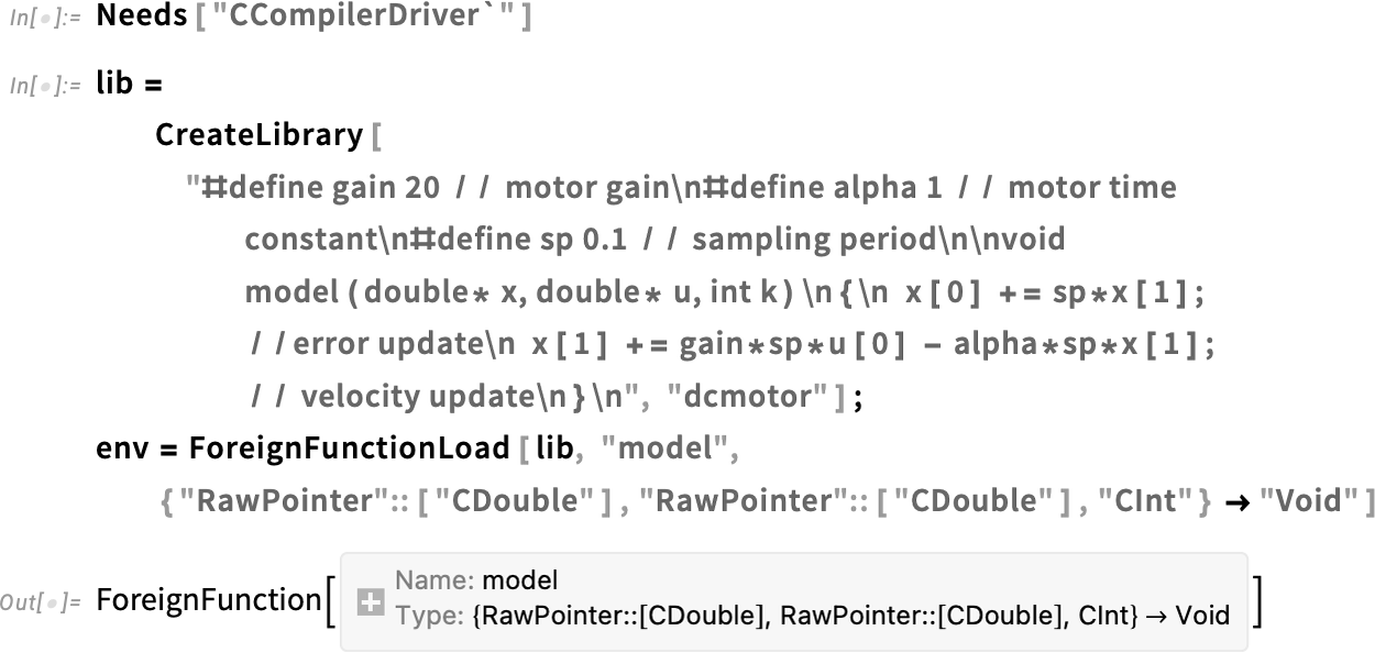
Now we can train a regulator for this (simulated system):
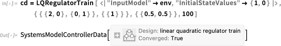
And, yes, this controller succeeds in bringing our simulated position error to zero:
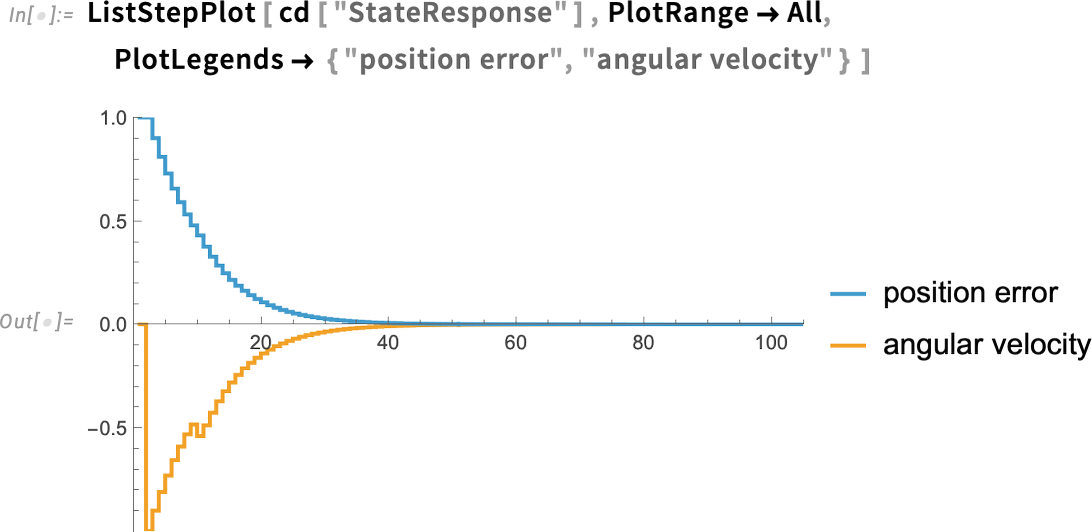
Importing & Exporting the Latest Formats
We first introduced streamlined importing and exporting of data with Import and Export more than 25 years ago. At the beginning we were dealing with a few tens of formats. Over time that number has grown to nearly 300. And as the years go by, there are always new formats that get defined or become popular. So in Version 15, for example, we’re introducing import and export of TOML and YAML, two simple formats that have become increasingly popular for configuration files of various kinds.
In the world of image formats, first there was GIF, then JPEG, then PNG. And now—with better modeling and representation of images—there’s HEIF and AVIF. And in Version 15 we now have full support for HEIF and AVIF for both importing and exporting, on all platforms—typically reducing the size of images at a given quality level by about a factor of two.
In the past few years we’ve been getting deeper and deeper support in Wolfram Language for astronomy and astronomical data. And as part of that, in Version 15 we’re introducing import for AVM—a metadata standard for astronomical images that specifies where a given image comes from in the sky, and how it was acquired.
A format that has been gaining in popularity in recent years is Markdown (.md). We first introduced import and export of Markdown in Version 14.2 and Version 14.3
respectively. In Version 15 we’re extending our Markdown support to include links, images, tables, etc. And in all cases we’re able both to get computable data in the form of associations, datasets, etc. as well as fully formatted notebooks.
In contrast to Markdown, with its fairly recent popularity, we have XML—which we’ve supported since 2002. XML tends to be a complex, if flexible, format. And in Version 15 we’ve added the capability to import XML directly as a computable Tree object.
Talking of old formats, there are notebooks, which, yes, we originally invented back in 1987 for Mathematica 1.0. We’ve been steadily developing and polishing the concept of notebooks for the four decades since—with all sorts of new features being added even in Version 15. Rather impressively, we’ve maintained compatibility though, so that Version 15.0 can still open a Version 1.0 notebook. But nearly a quarter century after we first invented notebooks, people finally started to copy them (why did it take so long?)—or, more accurately, copied some of their superficial features. But the end result is that there are some other notebook formats out in the world—and in Version 15 we’ve added the capability to import two of these—.vsnb and .ipynp—into our notebooks. (And, yes, export from our notebooks doesn’t make much sense; too much is missing in the “knock-off” notebook formats.)
Real-Time Connection with Web Sockets
How does one get data that’s being streamed from a server—and maybe respond to it as well? The basic mechanism—that’s existed in the world at large for decades—is to use sockets. A decade ago we introduced support for TCP sockets; later we added support for ZMQ sockets. And now in Version 15.0 we’re adding support for web sockets.
Web sockets are used for example in streaming data services, and in getting streamed results, say from cloud-based LLMs. An important feature of web sockets is that they’re bidirectional: even as data is being streamed to you, you can be sending data back to a server. Another important feature of web sockets is that their initial connection is made through http (or https), so that they can inherit all the various capabilities associated with http headers (like being able to pass in API keys, etc.).
Here’s a very simple example, based on the standard echo.websocket.org test socket. Here’s how we connect to this socket:
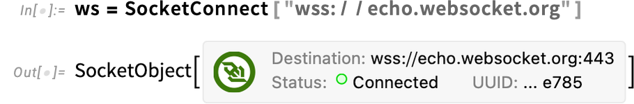
Now we can read from the socket—picking up the initial message that this particular server sends:
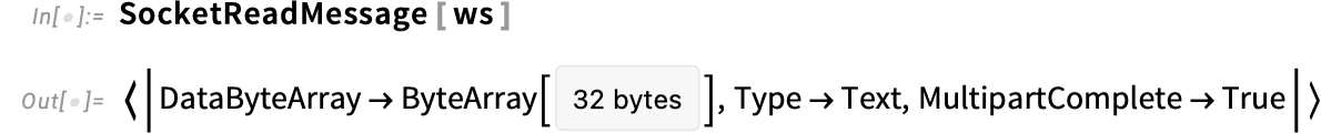
With SocketWriteMessage and SocketListen, we can then send messages back and forth. Our whole socket system works asynchronously, appropriately interacting with Dynamic to get updates as soon as they come in.
As a more complicated example, here’s how we would open a web socket connection to the current version of an OpenAI LLM system:
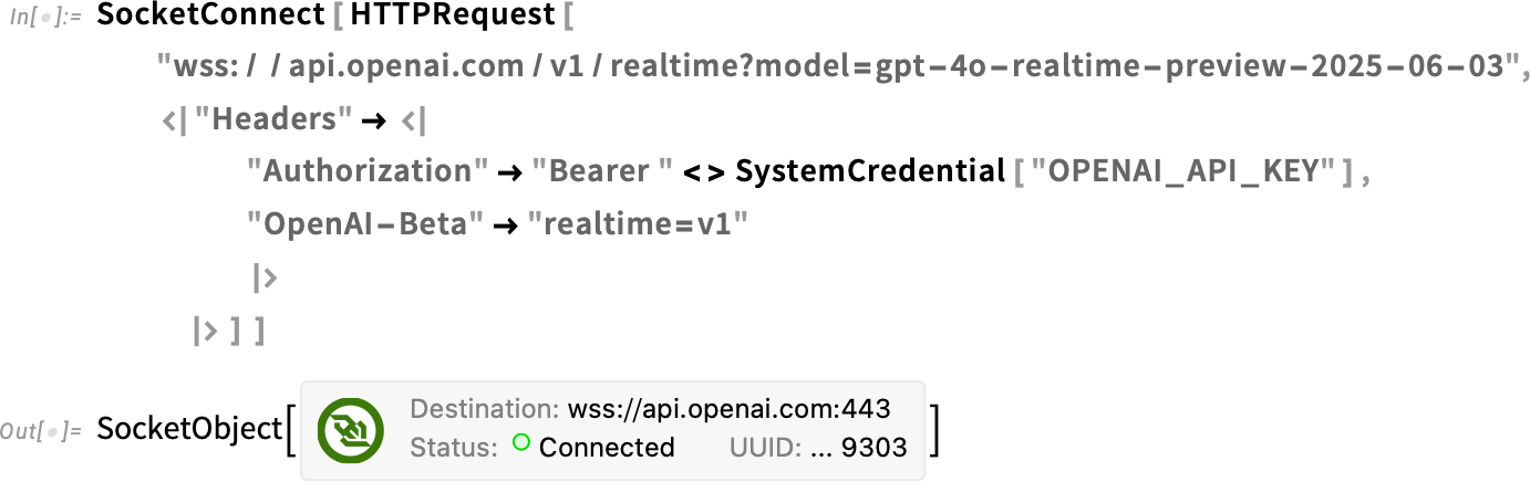
And, yes, in our AI Assistant—as well as Chat Notebooks, etc.—we are now going to be using web sockets to get real-time streamed results.
Richer UX for Using Python & More in Notebooks
Back in 2018 (in Version 11.3) we introduced external code cells to make it possible to include—and run—external code directly in notebooks. Type > at the beginning of a cell to get a menu of possible types of code:

Select Python and you’ll get a Python cell. But in Version 15 there’s something new here:

The external code cell is annotated with a “session menu”:

What’s the point of this? A single notebook can be connected to multiple different, independent Python sessions, and the session menu lets you manage these, and specify which one a particular cell should use.
Why should you need multiple Python sessions? Well, if Python was a nice coherent system like Wolfram Language you probably wouldn’t. But it’s not. And instead most functionality comes from a zoo of independently developed libraries, and it’s very common for different pieces of Python code to need different and incompatible sets of libraries. And, yes, if you just use Wolfram Language you avoid all of this mess. But if you already have code in Python (and, for example, an LLM can’t conveniently just translate it to Wolfram Language) then our external evaluation mechanism is set up to make integrating the Python code as painless as possible.
An important part of that is the encapsulation mechanism we introduced in Version 14.0 (and majorly enhanced in Version 14.3), that gives one the ability to have separate, fully-encapsulated Python sessions that carry and manage their own dependencies. Now in Version 15.0—with the session menu—we’re introducing a convenient interface to these encapsulated sessions.
Let’s say there’s a session with certain dependencies that’s already been set up. Now with our new session menu system you can choose that session as the one you want to use for a particular external code cell. For example, this sets up an external session with a particular dependency:
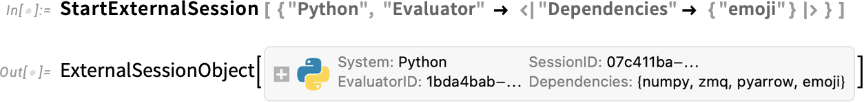
In the session menu for an external code cell you can now ask to Use a running Python session—and then pick this session:

Sessions can be explicitly named. But the default is that every newly created session gets a unique UUID. And that makes something very nice possible: it makes external code cells with dependencies transportable.
Here’s an external code cell using the session we set up:

But now the point is that this cell is in effect completely self contained. You can take it to another computer, send it to someone else, etc., and it’ll carry its dependencies with it, so that the Python code in it will just run.
In addition to defining Python sessions programmatically using StartExternalSession, you can also do it interactively, by directly picking Use a new Python session in the session menu.
The session menu for Python in Version 15 also has another couple of useful utility items. There’s Format code which applies automatic code formatting rules:

And there’s also Remove unused imports which determines what the actual dependencies of a piece of code are, and remove any unnecessary imports.
Optimization & GPUification Continues
The Wolfram Language is full of algorithmically complex functions, which we’re continually making more and more efficient. Some of our increased efficiency comes from using new algorithms (including many that we invent ourselves); some comes from being able to support additional hardware acceleration, notably with GPUs.
In Version 15 there are lots of performance enhancements throughout the system. And—for users with NVIDIA GPUs—there’s additional (experimental) acceleration of both core linear algebra and core graph theory functionality. With Method→"HybridCPUGPU", functions like LinearSolve automatically use both CPU and GPU hardware, achieving dramatic performance increases for cases like 10000×10000 matrices.
One of the issues in making efficient use of GPUs is being able to have the data they operate on resident in GPU memory. In Version 14.2 we introduced GPUArray as a way to specifically store data in GPU memory. And with each successive version we’re setting up more functions to operate directly on GPUArray objects.
In Version 15 we’ve added a collection of GPU-based array rearrangement functions. Here’s a 2000×2000 GPU array:
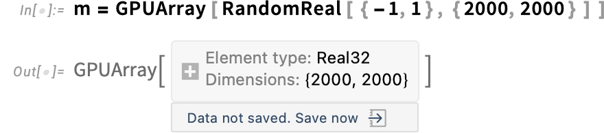
And assuming your computer has an appropriate GPU, this then very efficiently produces a GPU array, which, complicatedly enough, is a very different shape from the original:
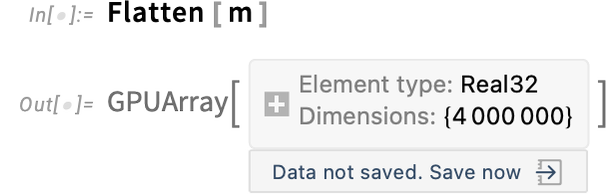
Using GPUs is still a fairly fiddly business, with different capabilities on different GPUs and different computer systems. We’re systematically implementing more and more functions for more and more GPU configurations, in each case setting up highly optimized GPU kernels.
And indeed, even beyond GPUs, there are complicated issues in different kinds of support with different hardware. So, for example, in Version 15 we’re adding Method![]() "MUMPS" for LinearSolve for sparse arrays, dramatically speeding up things like large-scale numerical PDE solving for ARM, Apple, etc. processors.
"MUMPS" for LinearSolve for sparse arrays, dramatically speeding up things like large-scale numerical PDE solving for ARM, Apple, etc. processors.
CUDA Kernels as External Functions
What if you want to write your own GPU code, and integrate it into the Wolfram Language? In Version 15.0 there’s a new mechanism for creating ExternalFunction objects that execute CUDA kernels. And, yes, this only works on systems that support CUDA, and have an appropriate GPU installed. Here’s an example where we’re giving pure CUDA C++ code, and getting an ExternalFunction that executes that code:
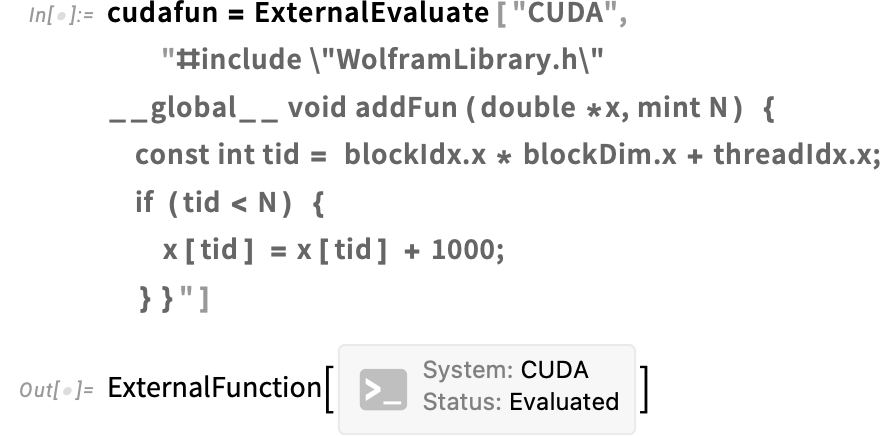
Now let’s say you set up a GPUArray—that will be resident on your GPU:
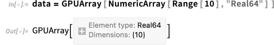
This runs the CUDA function on this array:
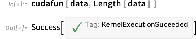
Here’s the result (and, yes, this particular CUDA kernel does the rather trivial thing of adding 1000 to each array element):
CUDA code tends to be very low level and rapidly gets quite involved and complicated. But in Version 15.0 there’s another way to do GPU programming: use Wolfram Language with the Wolfram Compiler, calling intrinsic CUDA functions using LibraryFunction. As an example, here’s a version of the same CUDA kernel as above, but now implemented in Wolfram Language using the Wolfram Compiler:
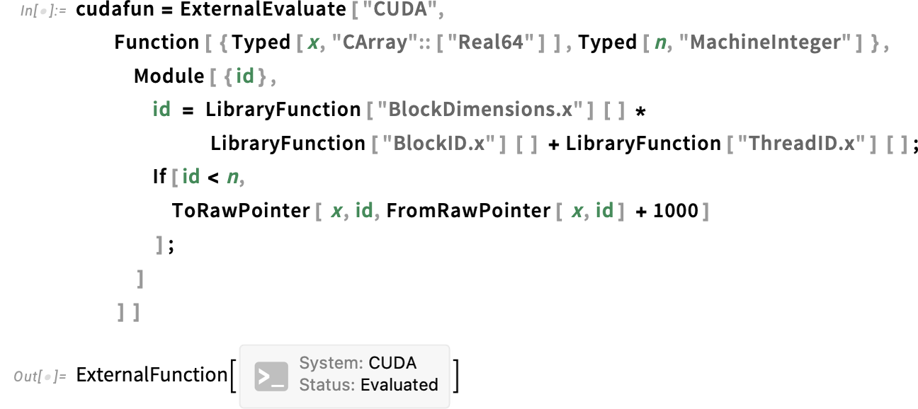
Now—just like with our raw CUDA code above—we can run this and get the result:

Wolfram Compute Services Gets GPUs
Late last year we launched Wolfram Compute Services—to make possible seamless large-scale remote computation. In the last few months we’ve added several features to Wolfram Compute Services, that are now fully integrated in Version 15. In particular, Wolfram Compute Services can now make use not only of CPUs, but also high-end GPUs.
As soon as you have your Wolfram Language code working, you can send it to Wolfram Compute Services just using RemoteBatchSubmit. Here we’ve got some neural net training that we’re submitting to be run on an NVIDIA L40S GPU:
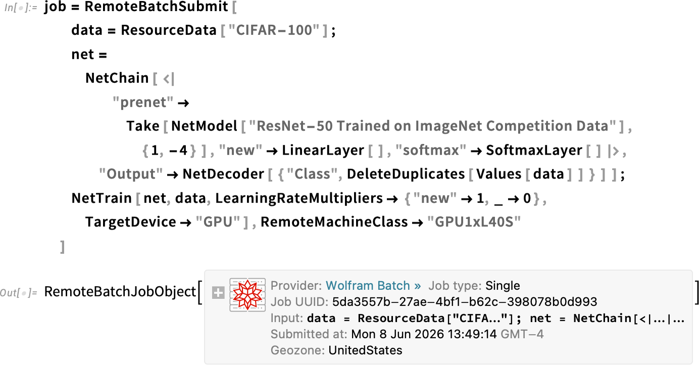
About 40 minutes later, we get an email saying the results are ready

and then we can retrieve them:
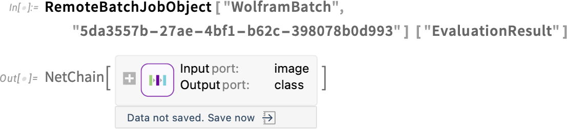
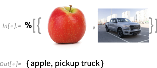
Another new feature in Wolfram Compute Services is the option RemoteGeoZone, which says where in the world the remote computation should be done—with "UnitedStates" and "EuropeanUnion" as the choices so far.
Wolfram Compute Services is set up to use public cloud infrastructure. But something we have under development is our High-Performance Computing Kit, which will allow private clusters and other institutional or organizational infrastructure to be set up to work with RemoteBatchSubmit.
We recently released our Wolfram Foundation Tool for LLM systems, that lets LLM systems access the power of the Wolfram Language, the Wolfram Knowledgebase, Wolfram|Alpha, etc. The core technology that makes this possible is what we call computation-augmented generation (CAG), a kind of infinite analog of retrieval-augmented generation (RAG) in which we’re doing real-time computations to supplement the capabilities of LLMs. Our Notebook Assistant (now AI Assistant) was already making use of a version of CAG and our Foundation Tool system. But in Version 15.0 we’ve extended this to all LLM functions. So now you can access any of our Foundation Tool family of capabilities by specifying an appropriate LLMEvaluator setting.
For example, here we’re using LLMSynthesize with the complete Wolfram Agent One LLM + Foundation Tool system to get a result that partly comes from an LLM, and partly from Wolfram Language computation:
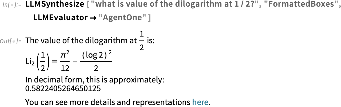
(You can also use LLMEvaluator → "AgentOne" in LLMFunction, ChatEvaluate, LLMGraph, etc.)
By the way, you can always specify your default LLMEvaluator by setting $LLMEvaluator, or by giving this in the Preferences panel.
Another useful setting for LLMEvaluator is "WolframAIAssistant". This gives access to the CAG system used for the interactive AI Assistant, that’s particularly geared to helping people write Wolfram Language code. Here, for example, we’re programmatically generating information about how to do something in Wolfram Language:
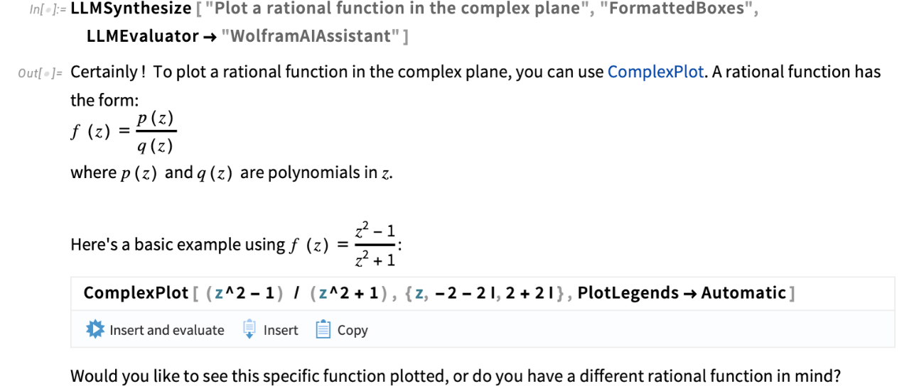
And Yet More…
In addition to everything we’ve already discussed, there are also all sorts of other new things in Version 15. Some are extensions and optimizations of existing functions; some are yet more entirely new functions.
For example, there’s PopovDecomposition and OrderedSchurDecomposition: two additional matrix decompositions. And there’s PfaffianDet, which computes the Pfaffian of an antisymmetric matrix:

Rounding out our large collection of integral transforms, Version 15 introduces DiscreteHilbertTransform (here of what amounts to a delta function):
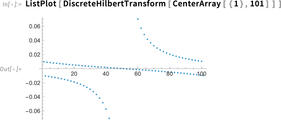
In graphs, we’ve made sure that PlanarFaceList lists the “outer face” of a planar graph first:
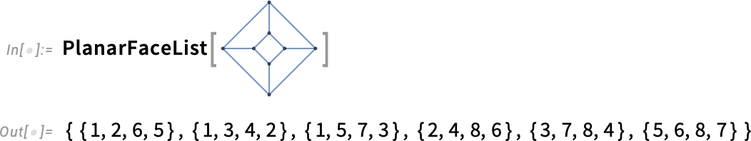
and there’s an option if you don’t want it:
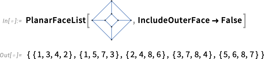
In graph layouts, there are several updates. First, there are new built-in styles for graph highlights, like “halo highlighting”:
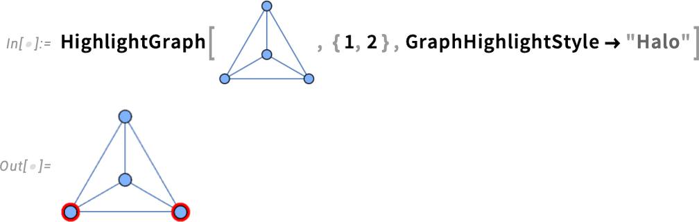
As well as new built-in edge shape functions—here delivering a rather ornate look:
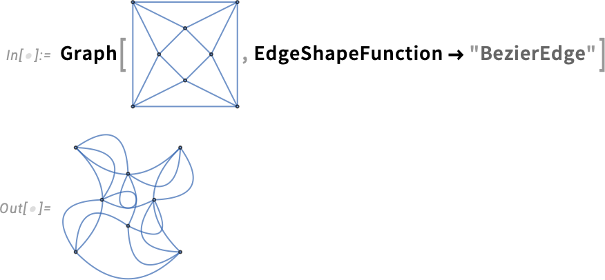
How does one represent smooth 3D surfaces? For nearly 20 years we’ve had BSplineSurface as a way to do this. In Version 15—as part of our effort to round out our tools for CAD-style geometry—we’re also introducing BezierSurface:
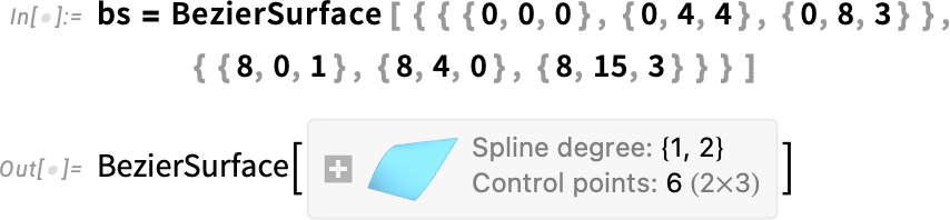
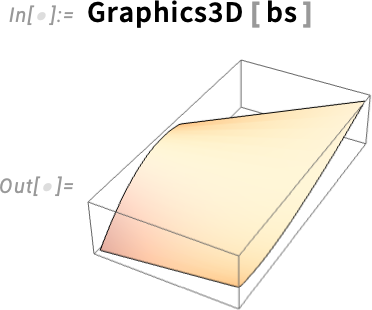
In a quite different area, Version 15 continues our development of chemistry capabilities, notably introducing MoleculeSubstructure for representing substructures in molecules. This finds cases of a particular molecular pattern within a molecule:
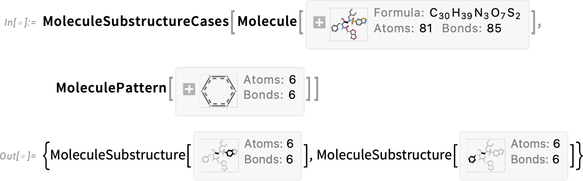
And this then plots these substructures:
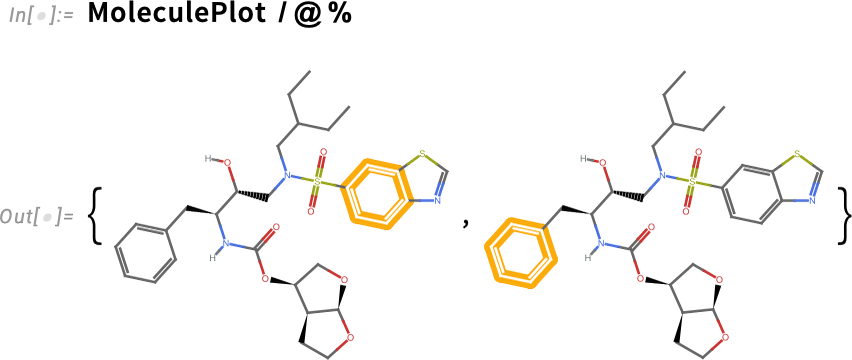
Also new in Version 15 is MoleculeFingerprint as well as MoleculeValue properties for stereochemistry.
There’s a lot more in Version 15 that we could discuss. But in an “always shoot for the Moon” moment I thought I’d finish with a new feature in Version 15 related to the Moon. More than a decade ago we introduced NightHemisphere (and DayHemisphere) to show day and night on maps:
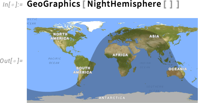
Well, now we’ve extended that capability “off planet”:
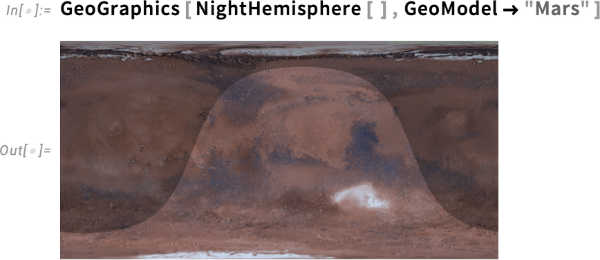
And, of course, to the Moon. To see what the Moon looks like to us from the Earth, we need to use an orthographic projection:
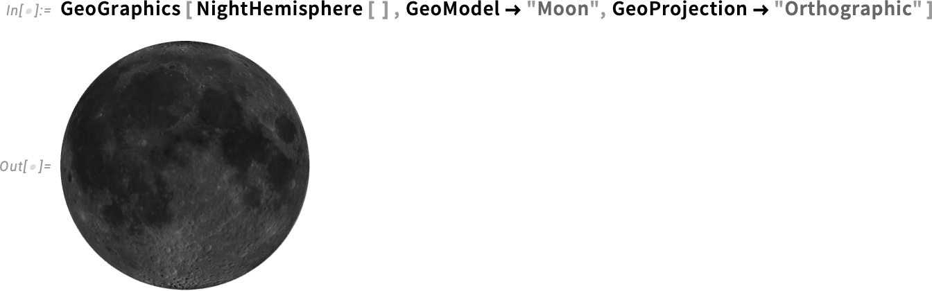
But what is this? Where is the day-night terminator? But then I realize: today is a new moon!
Everything is working as it should. And we’re carefully filling in yet another detail. And, yes, in another week it’ll be a quarter moon:
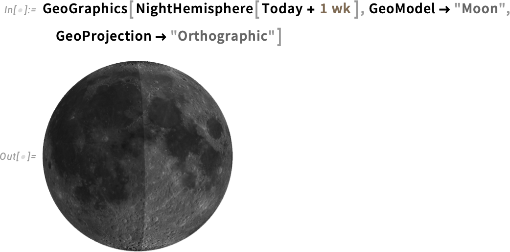


Add Comment